from sklearn.datasets import load_breast_cancer
data = load_breast_cancer()Getting Started

This page is a Jupyter notebook: text and Python code that you can run. You can read it here, run it on your own computer, or run it in your browser with the “Open in Colab” button (fine for a quick look, but Colab forgets the files you create). To run the notebooks on your computer, first follow Set Up Your Computer. The Course Guide explains how the course works and in which order to work through it.
On the What is Machine Learning? page you trained models by hand: you chose a model, measured its cost and moved the sliders until the cost was as low as possible. From now on you will do the same in code, with scikit-learn, one of the most widely used Python libraries for machine learning. Scikit-learn searches for the best parameters for you, so you can focus on the data, the choice of model and checking the predictions on test data.
In this notebook you get to know the datasets used in the self-study notebooks, and their features and labels, which scikit-learn calls X and y. In the next notebooks you will train your first classification and regression models on them.
To learn how to build machine learning models with scikit-learn, focus on two activities:
- Explore the scikit-learn documentation: it not only explains how scikit-learn works but also showcases powerful examples you can learn from
- Write code yourself: “Knowing is not enough; we must apply.” said someone very smart.
On NumPy, Pandas, and Matplotlib
These are the core libraries of data science. You should already know their basics (see the prerequisites on the course homepage), but their possibilities are nearly endless. Rather than memorizing every method, what truly matters is knowing what’s possible and having the skill to use any method you haven’t seen before by reading its documentation.
We won’t offer a separate “advanced” course, instead, you’ll keep expanding your mastery through real use cases as they arise in the self-study notebooks. Whenever you encounter a new function or method, treat it as an opportunity to strengthen this essential skill: learning directly from documentation. Of course, you can always use LLMs to explain you a method. However, keep in mind that, LLMs are not always up-to-date with the documentations.
The datasets
To build and evaluate machine learning models, we need data. The scikit-learn library provides several well-known datasets that are ideal for learning and experimentation. We will use a selection of these datasets during the self-study.
Scikit-learn provides 4 types of datasets:
In the self-study notebooks, we will use the following five datasets, from toy, real, and external datasets:
- Breast cancer Wisconsin (diagnostic) dataset (binary classification)
- Vehicle dataset (multi-class classification)
- fetch_openml documentation
- Use
X, y = fetch_openml(name="vehicle", version=1, as_frame=True, return_X_y=True)
- Diabetes dataset (regression)
- California Housing dataset (regression)
- Palmer penguins dataset (multi-class classification, and regression)
- Use
X, y = fetch_openml(name="penguins", version=1, as_frame=True, return_X_y=True)
- Use
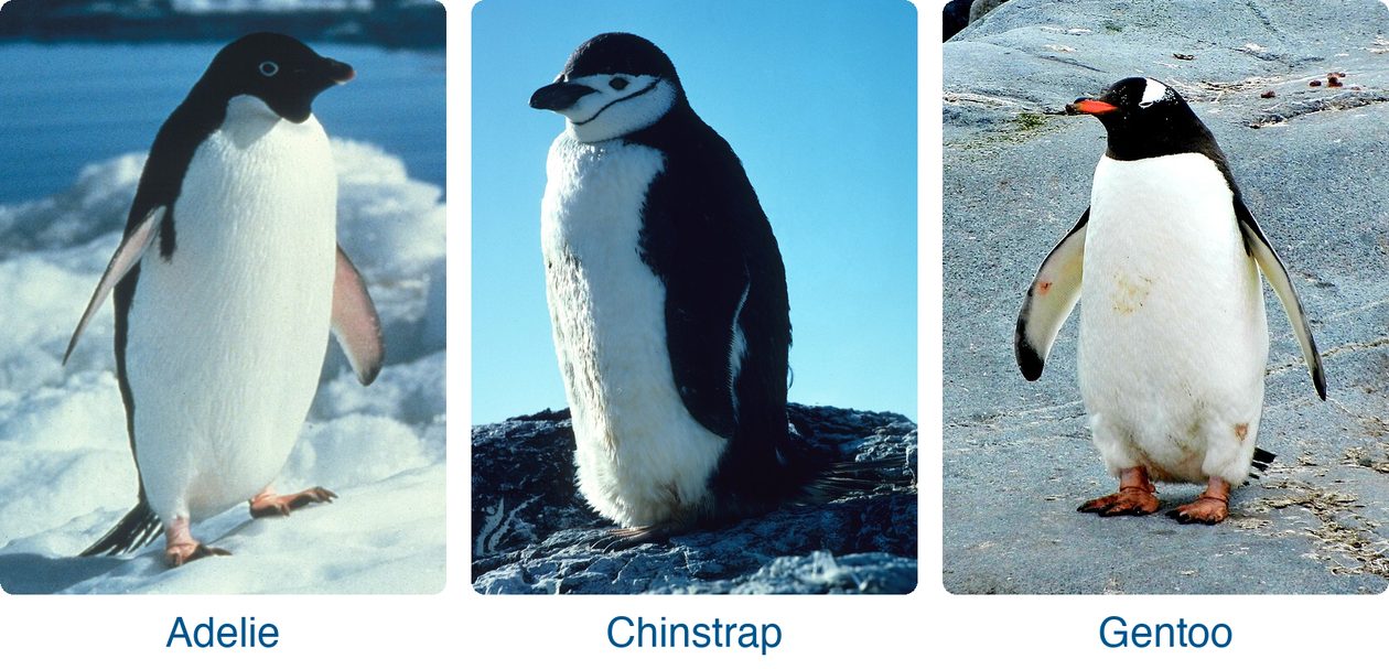
The Palmer penguins dataset has measurements of 344 penguins of three species, Adelie, Chinstrap and Gentoo, on three islands in Antarctica. Dr. Kristen Gorman and the Palmer Station Long Term Ecological Research program collected the data. The self-study notebooks use it to predict the species of a penguin (classification) and its body mass (regression).
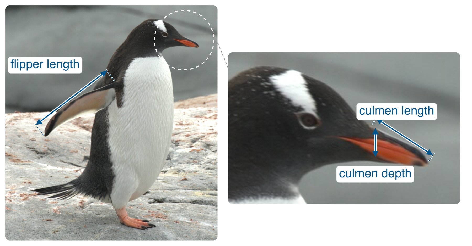
Three of the measurements are lengths in millimeters: the length of the flipper (wing), and the length and depth of the culmen, the upper ridge of the bill:
you can load scikit-learn datasets very easily. Let’s load the first dataset. Go to the documentation of the Breast cancer dataset, scroll down to find the examples sections, which tells you how to load the dataset:
but what is data? Again the documentation:
Returns:
    data: Bunch
        Dictionary-like object, with the following attributes.

        data: {ndarray, dataframe} of shape (569, 30)
            The data matrix. If as_frame=True, data will be a pandas DataFrame.
...
# since it is a dictionary like object
# we can check the keys
data.keys()dict_keys(['data', 'target', 'frame', 'target_names', 'DESCR', 'feature_names', 'filename', 'data_module'])# this is a numpy array
data['data']array([[1.799e+01, 1.038e+01, 1.228e+02, ..., 2.654e-01, 4.601e-01,
1.189e-01],
[2.057e+01, 1.777e+01, 1.329e+02, ..., 1.860e-01, 2.750e-01,
8.902e-02],
[1.969e+01, 2.125e+01, 1.300e+02, ..., 2.430e-01, 3.613e-01,
8.758e-02],
...,
[1.660e+01, 2.808e+01, 1.083e+02, ..., 1.418e-01, 2.218e-01,
7.820e-02],
[2.060e+01, 2.933e+01, 1.401e+02, ..., 2.650e-01, 4.087e-01,
1.240e-01],
[7.760e+00, 2.454e+01, 4.792e+01, ..., 0.000e+00, 2.871e-01,
7.039e-02]], shape=(569, 30))# these are the column names
data['feature_names']array(['mean radius', 'mean texture', 'mean perimeter', 'mean area',
'mean smoothness', 'mean compactness', 'mean concavity',
'mean concave points', 'mean symmetry', 'mean fractal dimension',
'radius error', 'texture error', 'perimeter error', 'area error',
'smoothness error', 'compactness error', 'concavity error',
'concave points error', 'symmetry error',
'fractal dimension error', 'worst radius', 'worst texture',
'worst perimeter', 'worst area', 'worst smoothness',
'worst compactness', 'worst concavity', 'worst concave points',
'worst symmetry', 'worst fractal dimension'], dtype='<U23')We can create a Pandas DataFrame to view each column with its header. However, if you read the documentation, you’ll notice that load_breast_cancer() can directly return the data as X and y (explained below).
This function has two useful parameters: return_X_y and as_frame. Read what they do in the documentation, then check the code below to see their effect.
X, y = load_breast_cancer(as_frame=True, return_X_y=True)In machine learning, it is a common convention to use X and y to represent the data:
- X (uppercase) refers to the input features — the independent variables used by the model to make predictions. It is typically a table or matrix where each row is a data sample and each column is a feature.
- y (lowercase) refers to the target variable — the value we want to predict. It can be categorical (for classification) or continuous (for regression).
This convention helps keep code consistent and readable across different datasets and models.
# X is a pandas DataFrame containing the feature variables,
# and y is a pandas Series containing the target variable.
type(X), type(y)
(pandas.DataFrame, pandas.Series)X.head()| mean radius | mean texture | mean perimeter | mean area | mean smoothness | mean compactness | mean concavity | mean concave points | mean symmetry | mean fractal dimension | ... | worst radius | worst texture | worst perimeter | worst area | worst smoothness | worst compactness | worst concavity | worst concave points | worst symmetry | worst fractal dimension | |
|---|---|---|---|---|---|---|---|---|---|---|---|---|---|---|---|---|---|---|---|---|---|
| 0 | 17.99 | 10.38 | 122.80 | 1001.0 | 0.11840 | 0.27760 | 0.3001 | 0.14710 | 0.2419 | 0.07871 | ... | 25.38 | 17.33 | 184.60 | 2019.0 | 0.1622 | 0.6656 | 0.7119 | 0.2654 | 0.4601 | 0.11890 |
| 1 | 20.57 | 17.77 | 132.90 | 1326.0 | 0.08474 | 0.07864 | 0.0869 | 0.07017 | 0.1812 | 0.05667 | ... | 24.99 | 23.41 | 158.80 | 1956.0 | 0.1238 | 0.1866 | 0.2416 | 0.1860 | 0.2750 | 0.08902 |
| 2 | 19.69 | 21.25 | 130.00 | 1203.0 | 0.10960 | 0.15990 | 0.1974 | 0.12790 | 0.2069 | 0.05999 | ... | 23.57 | 25.53 | 152.50 | 1709.0 | 0.1444 | 0.4245 | 0.4504 | 0.2430 | 0.3613 | 0.08758 |
| 3 | 11.42 | 20.38 | 77.58 | 386.1 | 0.14250 | 0.28390 | 0.2414 | 0.10520 | 0.2597 | 0.09744 | ... | 14.91 | 26.50 | 98.87 | 567.7 | 0.2098 | 0.8663 | 0.6869 | 0.2575 | 0.6638 | 0.17300 |
| 4 | 20.29 | 14.34 | 135.10 | 1297.0 | 0.10030 | 0.13280 | 0.1980 | 0.10430 | 0.1809 | 0.05883 | ... | 22.54 | 16.67 | 152.20 | 1575.0 | 0.1374 | 0.2050 | 0.4000 | 0.1625 | 0.2364 | 0.07678 |
5 rows × 30 columns
y.head()0 0
1 0
2 0
3 0
4 0
Name: target, dtype: int64This is the Breast Cancer Wisconsin dataset. In this dataset, each row represents one patient, and the data describe characteristics of a breast tumor found in that patient. The input data (X) contain 30 features, which are numerical measurements describing the tumor’s shape, size, texture, and other properties obtained from medical images. The target variable (y) tells us whether the tumor is malignant (0), meaning cancerous, or benign (1), meaning not cancerous.
There are 569 patients in total, with 357 benign and 212 malignant cases. The goal of a machine learning model is to learn from these examples so that, given the measurements of a new tumor, it can predict whether it is likely to be benign or malignant. Note that in machine learning, the term “positive class” simply means the class labelled 1 (here, benign = 1), not that it is “positive” in a good or bad sense. Some later notebooks flip the labels so that malignant is 1, the class they want to detect; they say so when they do.
# 569 patients (i.e. tumors), 30 features
X.shape
(569, 30)# 212 tumors are labeled as malignant (0)
# 357 tumors are labeled as benign (1)
y.value_counts() # very useful to know this method, instead of writing a loop to counttarget
1 357
0 212
Name: count, dtype: int64I’ve demonstrated how to read the documentation and adjust your code accordingly. From this point on, I won’t show these steps for every example, part of your learning is to practice finding, reading, and applying documentation on your own.
On the documentation page:
https://scikit-learn.org/stable/modules/generated/sklearn.datasets.load_breast_cancer.html#sklearn.datasets.load_breast_cancer
you’ll also see a line that says “Read more in the User Guide.” Click that link to explore detailed information about the dataset, which should take you here:
https://scikit-learn.org/stable/datasets/toy_dataset.html#breast-cancer-dataset
# Gives summary statistics for all features in X, such as mean, standard deviation, min, max, and quartiles.
X.describe()| mean radius | mean texture | mean perimeter | mean area | mean smoothness | mean compactness | mean concavity | mean concave points | mean symmetry | mean fractal dimension | ... | worst radius | worst texture | worst perimeter | worst area | worst smoothness | worst compactness | worst concavity | worst concave points | worst symmetry | worst fractal dimension | |
|---|---|---|---|---|---|---|---|---|---|---|---|---|---|---|---|---|---|---|---|---|---|
| count | 569.000000 | 569.000000 | 569.000000 | 569.000000 | 569.000000 | 569.000000 | 569.000000 | 569.000000 | 569.000000 | 569.000000 | ... | 569.000000 | 569.000000 | 569.000000 | 569.000000 | 569.000000 | 569.000000 | 569.000000 | 569.000000 | 569.000000 | 569.000000 |
| mean | 14.127292 | 19.289649 | 91.969033 | 654.889104 | 0.096360 | 0.104341 | 0.088799 | 0.048919 | 0.181162 | 0.062798 | ... | 16.269190 | 25.677223 | 107.261213 | 880.583128 | 0.132369 | 0.254265 | 0.272188 | 0.114606 | 0.290076 | 0.083946 |
| std | 3.524049 | 4.301036 | 24.298981 | 351.914129 | 0.014064 | 0.052813 | 0.079720 | 0.038803 | 0.027414 | 0.007060 | ... | 4.833242 | 6.146258 | 33.602542 | 569.356993 | 0.022832 | 0.157336 | 0.208624 | 0.065732 | 0.061867 | 0.018061 |
| min | 6.981000 | 9.710000 | 43.790000 | 143.500000 | 0.052630 | 0.019380 | 0.000000 | 0.000000 | 0.106000 | 0.049960 | ... | 7.930000 | 12.020000 | 50.410000 | 185.200000 | 0.071170 | 0.027290 | 0.000000 | 0.000000 | 0.156500 | 0.055040 |
| 25% | 11.700000 | 16.170000 | 75.170000 | 420.300000 | 0.086370 | 0.064920 | 0.029560 | 0.020310 | 0.161900 | 0.057700 | ... | 13.010000 | 21.080000 | 84.110000 | 515.300000 | 0.116600 | 0.147200 | 0.114500 | 0.064930 | 0.250400 | 0.071460 |
| 50% | 13.370000 | 18.840000 | 86.240000 | 551.100000 | 0.095870 | 0.092630 | 0.061540 | 0.033500 | 0.179200 | 0.061540 | ... | 14.970000 | 25.410000 | 97.660000 | 686.500000 | 0.131300 | 0.211900 | 0.226700 | 0.099930 | 0.282200 | 0.080040 |
| 75% | 15.780000 | 21.800000 | 104.100000 | 782.700000 | 0.105300 | 0.130400 | 0.130700 | 0.074000 | 0.195700 | 0.066120 | ... | 18.790000 | 29.720000 | 125.400000 | 1084.000000 | 0.146000 | 0.339100 | 0.382900 | 0.161400 | 0.317900 | 0.092080 |
| max | 28.110000 | 39.280000 | 188.500000 | 2501.000000 | 0.163400 | 0.345400 | 0.426800 | 0.201200 | 0.304000 | 0.097440 | ... | 36.040000 | 49.540000 | 251.200000 | 4254.000000 | 0.222600 | 1.058000 | 1.252000 | 0.291000 | 0.663800 | 0.207500 |
8 rows × 30 columns
YOUR TURN
Real datasets often contain missing values. Check if X contains any missing values.
# YOUR CODE HEREBefore building a machine learning model on a dataset, it’s important to start with a clear understanding of the data and the problem you are trying to solve. Ask yourself the following key questions:
- What is the problem? What do I need to predict, and based on which input features?
- Type of problem: Is it a classification (predicting categories) or a regression (predicting continuous values) task?
- If classification: How many classes are there, and what are their value counts?
- If regression: Min-max value of the target? (going forward you need to check the distribution)
- Data size: How many rows (samples) and columns (features) does the dataset contain?
- Feature types: Which features are categorical and which are numerical?
- Data quality: Are there any missing values that need to be handled?
Answering these questions helps you understand your dataset and choose appropriate preprocessing steps and models.
Based on our code above, we can answer these questions for the Breast Cancer Wisconsin dataset.
- What is the problem? The goal is to predict whether a breast tumor is benign (not cancerous) or malignant (cancerous) based on measurements of the tumor.
- Type of problem: This is a classification problem because we are predicting one of two categories.
- If classification: There are 2 classes — malignant (0) and benign (1).
- Value counts per class: There are 212 malignant cases and 357 benign cases.
- Data size: The dataset has 569 rows (patients) and 30 columns (numerical features).
- Feature types: All 30 features are numerical, describing properties such as radius, texture, smoothness, and symmetry of the tumor.
- Missing values: The dataset does not contain any missing values.
YOUR TURN
Repeat the above process for the remaining 4 datasets.
- Vehicle dataset (multi-class classification)
- fetch_openml documentation
- Use
X, y = fetch_openml(name="vehicle", version=1, as_frame=True, return_X_y=True)
- Diabetes dataset (regression)
- California Housing dataset (regression)
- Palmer penguins dataset (multi-class classification: the species)
- Use
X, y = fetch_openml(name="penguins", version=1, as_frame=True, return_X_y=True)
- Use
Answer the following questions for each:
- What is the problem? What do I need to predict, and based on which input features?
- Type of problem: Is it a classification (predicting categories) or a regression (predicting continuous values) task?
- If classification: How many classes are there, and what are their value counts?
- If regression: Min-max value of the target?
- Data size: How many rows (samples) and columns (features) does the dataset contain?
- Feature types: Which features are categorical and which are numerical?
- Data quality: Are there any missing values that need to be handled?
# YOUR CODE HERE