from pathlib import Path
import numpy as np
import pandas as pd
import matplotlib.pyplot as plt
import matplotlib

print("pandas version:", pd.__version__)
print("numpy version:", np.__version__)
print("matplotlib version:", matplotlib.__version__)Classification

This is the first of the three notebooks of Iteration 1: Classification, Regression and Clustering. They build on each other, so do them in this order.
The goal of this notebook is not to master every detail of machine learning, but to understand the whole game. You’ll follow the complete CRISP-DM process, from Business Understanding to Evaluation, experiencing each phase in a simple and structured way. Deployment is the final phase of CRISP-DM; in this course it is limited to saving your trained model.
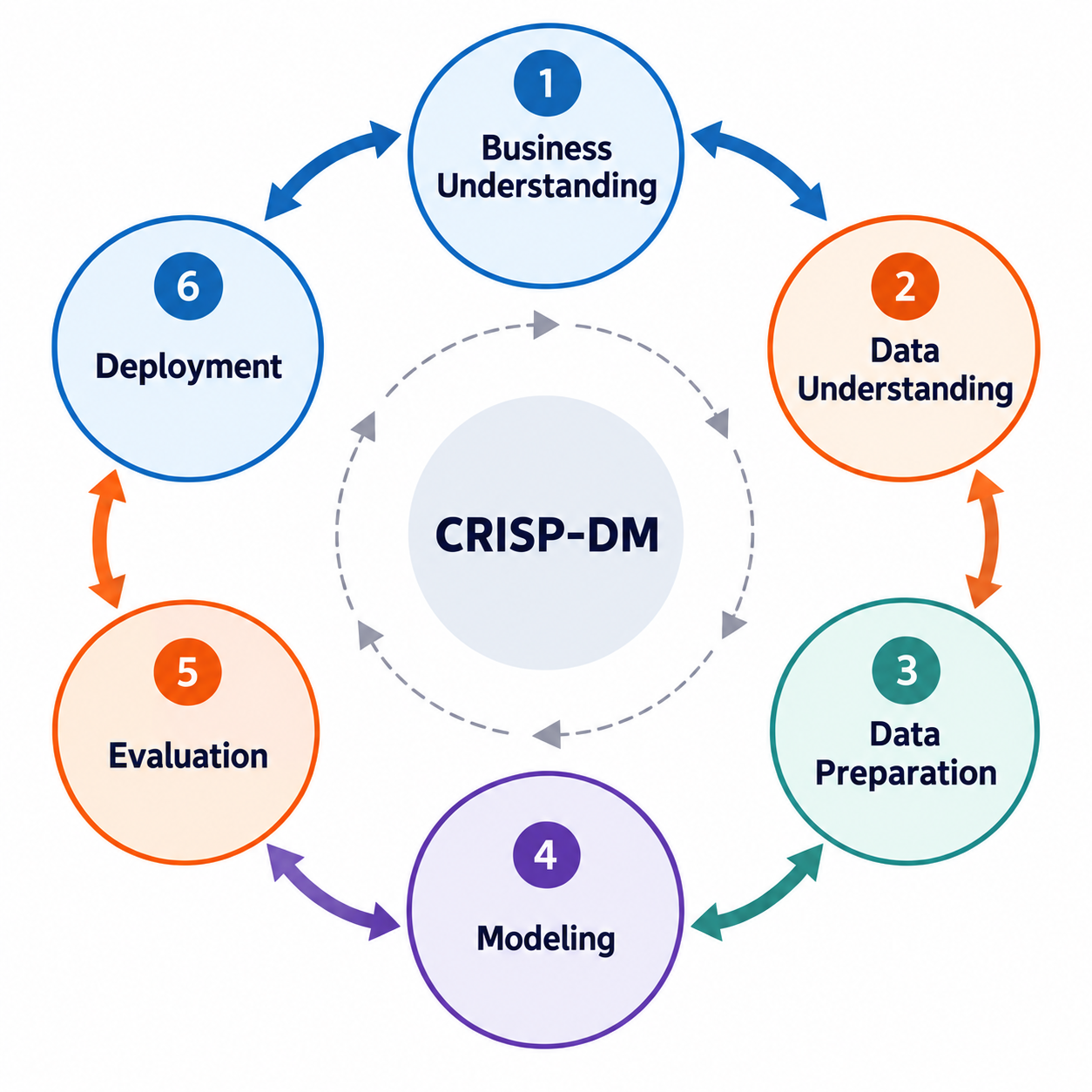
In this notebook you will work through the main phases of a data science project:
- Phase 1 – Business Understanding: ✅ You already completed it on the Business Understanding page.
- Phase 2 – Data Understanding: ✅ You read the Data Understanding page. In this notebook you continue with a hands-on exploration of the dataset.
- Phase 3 – Data Preparation: Prepare the dataset so it can be used for training models.
- Phase 4 – Modelling: Train a classification model to predict molecular stability.
- Phase 5 – Evaluation: Assess the performance of your trained model.
- Phase 6 – Deployment: Save the trained model for future use.
The goal here is not to perfect each step, but to connect them and see how the entire process fits together. By the end, you’ll have experienced the full machine learning workflow and gained insight into the lifecycle of a data science project.
Let’s get started!
1. Business Understanding
Done ✅ You read the Business Understanding page.
2. Data Understanding
Done ✅ You read the Data Understanding page. Now explore the dataset yourself. The Regression and Clustering notebooks use the same dataset and build on what you find here.
Your Turn
Read starter_dataset.xlsx as a pandas dataframe into the df variable. You can find it under data/002_processed_data.
Working in Colab? The repository’s
data/folder is not available there. Pandas can read the file directly from GitHub instead:pd.read_excel("https://raw.githubusercontent.com/BredaUniversityADSAI/introduction-to-ml/stable/data/002_processed_data/starter_dataset.xlsx")
# YOUR CODE HEREYour Turn
Use the df.info() method to explore the dataset, and answer the following:
- How many rows and columns does the dataset contain?
- How many numerical and how many text columns are there? (In pandas 3, the version of this course, text columns have the dtype
str; older versions, for example on Colab, showobject.)
# YOUR CODE HEREYour Turn
Use the df.describe() method to generate descriptive statistics for the dataset, then answer the following questions:
- Does the number of columns shown in the output match the total number of columns in the dataset?
- If not, why is there a mismatch? (For example, you might see 221 columns in total, but only 219 in the summary.)
# YOUR CODE HEREYour Turn
By default, the df.describe() method returns descriptive statistics for numerical columns only. Explore the documentation and identify the parameter that allows you to include all columns, including categorical ones, in the summary. Then, modify your code to display descriptive statistics for all columns in the dataset.
# YOUR CODE HEREYour Turn
Identify the non-numerical columns in the dataset and store their names in a list of strings.
# YOUR CODE HEREYour Turn
Check for missing values in the dataset. Count the number of NaN values in each column, and if a column contains any missing values, print its name along with the number of missing entries.
# YOUR CODE HEREYour Turn
First, locate the column names corresponding to the target variables. Then, determine whether each target variable should be treated as a regression or classification task.
# YOUR CODE HEREYour Turn
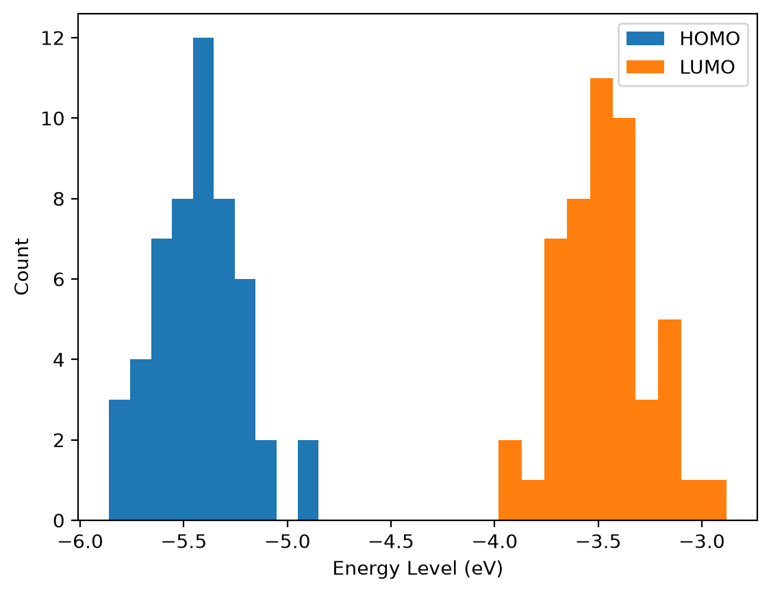
It is key for you to understand the distribution of target variables. Replicate the following plots:
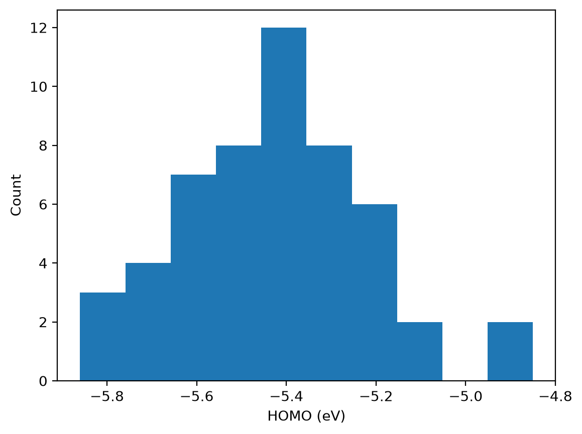
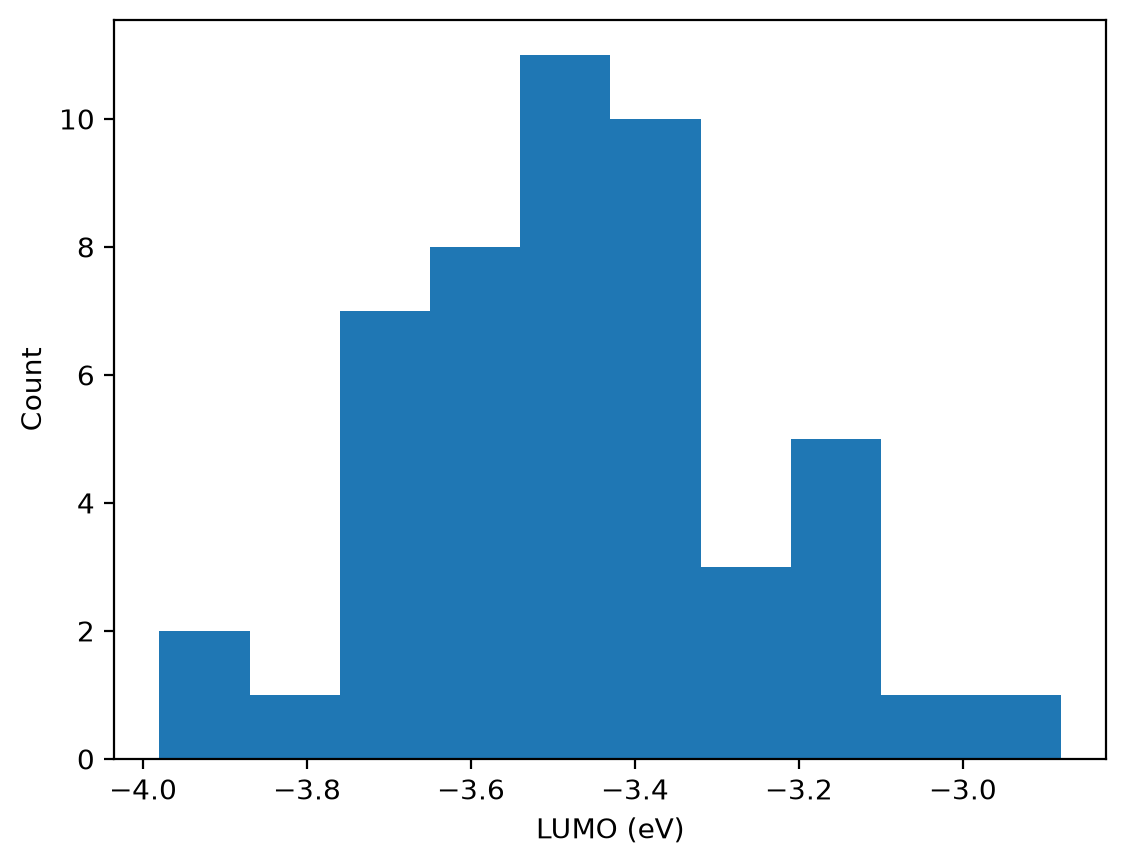
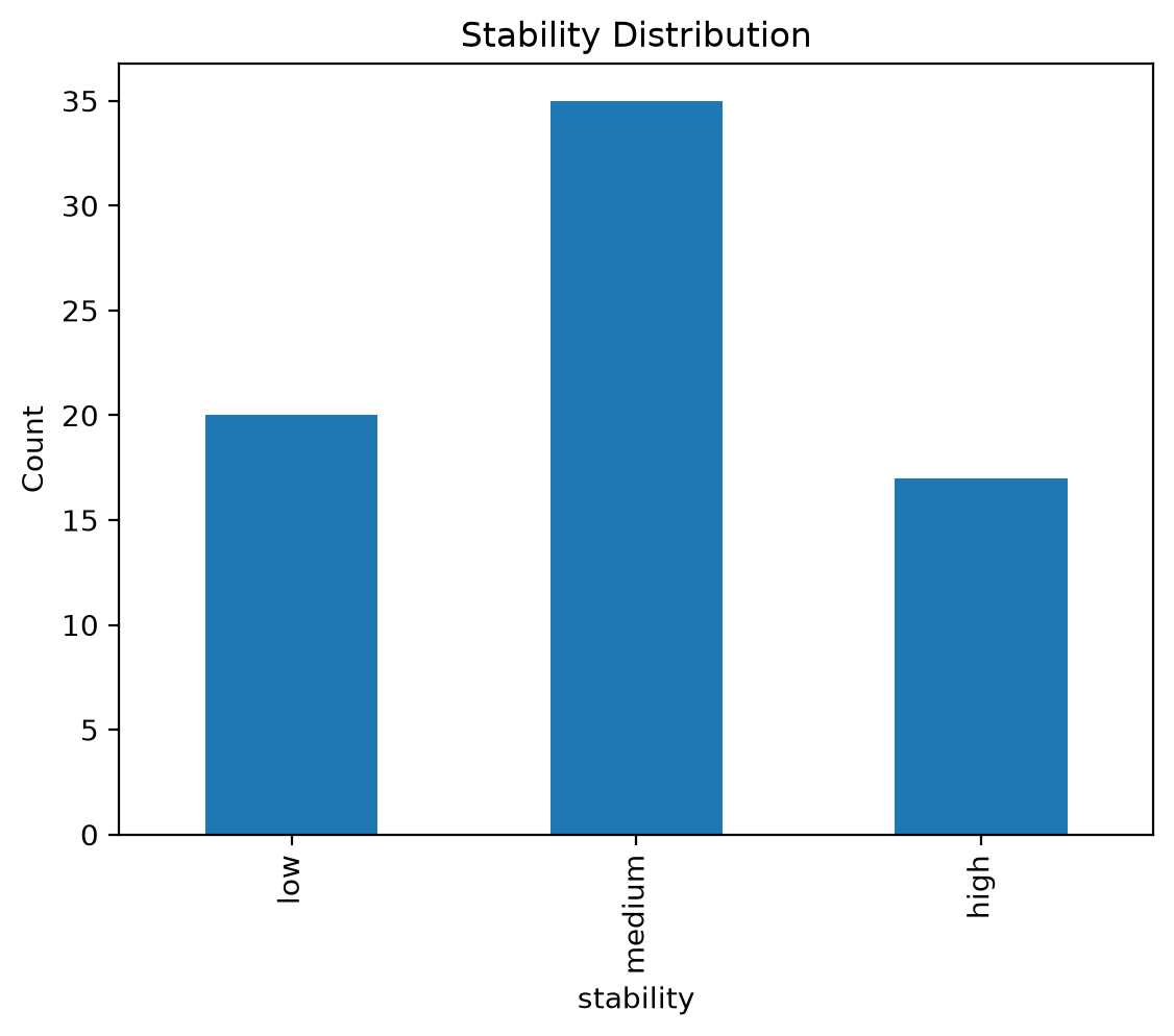
Note: Both HOMO and LUMO represent molecular orbital energy levels. As explained in the business understanding document, LUMO values are generally expected to be higher (i.e., closer to zero) than HOMO values. Let’s verify whether this pattern holds in our dataset.
# YOUR CODE HERE# YOUR CODE HERE# YOUR CODE HERE# YOUR CODE HERE3. Data Preparation
As explained in the Data Understanding section, the dataset is already prepared for you. Therefore this section will be short.
Your Turn
In this notebook you predict stability, so a row without a stability value is of no use for training or testing. Remove the rows where stability is missing (NaN). How many molecules are left?
Why not also remove the rows where homo or lumo is missing? Those columns are not used here, so you would throw away molecules that have a perfectly good label for this task.
# YOUR CODE HEREYour Turn
Many scikit-learn models expect numerical values as input, so non-numerical features can cause errors. In the starter_dataset.xlsx, all our input features are numerical.
- Keep the column
stabilityas it is, for classification, scikit-learn can handle string labels directly. - Drop the column
smiles, since it is not an input to the model.
# YOUR CODE HERE4. Modeling
df.head()Your Turn
Create the input features X by selecting the molecular descriptor columns, and set the target variable y to the stability column. You can do this by slicing the DataFrame so that X contains all descriptor columns and y contains only stability.
# YOUR CODE HEREBefore building a model, it is useful to establish a non-learning baseline. Your model should perform better than this baseline; otherwise, there is little point in training a model.
For classification with balanced classes, the random-guess baseline is simply \(1 / \text{num\_classes}\). For example, with 3 classes, random guessing would give about 33% accuracy.
For imbalanced classes, however, a stronger baseline is to always predict the majority class, the class with the highest frequency in the dataset. From the data understanding step, we know that the majority class here is "medium".
Your Turn
Calculate the accuracy you would achieve if you always predict "medium". For this first quick estimate you can use all of y. Strictly speaking, a baseline should be treated like a model: take the majority class from the training set only and measure its accuracy on the test set, so that it is compared with your model on the same data.
# YOUR CODE HEREYour Turn
Import train_test_split from sklearn.model_selection, and use it to split your data into training and test sets. The training set should contain 80 percent of the data and the test set the remaining 20 percent. Set random_state=42 to ensure reproducibility. Finally, check the shapes of X_train, y_train, X_test, and y_test to confirm the split worked correctly.
# YOUR CODE HEREYour Turn
Import the RandomForestClassifier from sklearn.ensemble, create a model instance with random_state=42 for reproducibility, and fit the model on the training data (X_train, y_train).
# YOUR CODE HERE5. Evaluation
In this section, you will assess the performance of your model. To do this, we use data that the model has not seen during training, that’s why we created a test set. Use X_test to generate predictions (y_pred), and then compare these predictions to the true labels (y_test).
Your Turn
Use the trained model’s .predict method with X_test and save the predicted labels in y_pred.
# YOUR CODE HEREYour Turn
Evaluate the model’s performance using scikit-learn’s built-in metrics. Import accuracy_score from sklearn.metrics, calculate the accuracy by comparing y_test and y_pred, and report the result in 3 decimal places.
# YOUR CODE HEREIs the model performing better than the baseline? Remember that your first model may not capture much. Through iterations, such as adding more data, refining features, tuning hyperparameters, or trying different algorithms, you should be able to surpass the baseline. If, after many attempts, the model still cannot beat the baseline, this may suggest that the dataset does not contain enough signal to learn from.
Your Turn
How much can you trust this comparison? Your test set holds only about 15 molecules, so one molecule more or less predicted correctly moves the accuracy by almost 7 percentage points.
Repeat the split, the training and the evaluation with random_state 0, 1, 2, 3 and 4 for train_test_split (keep random_state=42 for the model), and print the accuracy of each run. How large is the spread? Is your model better than the baseline in every run? In Iteration 3, after the Module 3 Self-study, you will use a more reliable way to estimate performance: cross-validation.
# YOUR CODE HEREYour Turn
While overall metrics like accuracy are useful, it’s also important to look at individual predictions to understand how the model behaves on specific cases. Create a DataFrame that compares the model’s predictions (y_pred) with the true labels (y_test). This will let you inspect individual results alongside the aggregate performance.
# YOUR CODE HERE6. Deployment
As mentioned at the beginning of this notebook, we will not go into the full deployment phase. Deployment refers to everything involved in making a model available for real users, and the very first step in that process is saving the trained model so it can be reused later.
Your task is to save the trained model, so that you can later use it to make predictions (inference) on new molecules, such as the course’s test molecules. Save your model in the models folder at the root of the course repository.
But before doing so, consider the following question:
Should you just save the model as it is? Or is there an extra step you should take?
Think about this for a moment before reading on.
When we did a train/test split, the purpose was to evaluate our model on unseen data. However, once we are done with testing and want to actually use the model (for example, to predict the test molecules), we might want to retrain it on the entire dataset. Training on all the data could potentially improve performance, since the model sees more examples, but the downside is that we no longer have a test set to estimate its accuracy.
In this course, the performance estimate can also come from the public score on the test molecules (from Iteration 3), which serves as feedback on how well your model does on molecules it has never seen.
Your Turn
- Retrain the model on the entire dataset (i.e. X and y instead of X_train, y_train)
- Use
joblib.dumpto save the model under the “models” folder asstability_iteration1.joblib
Here is the documentation for joblib.dump: https://joblib.readthedocs.io/en/stable/generated/joblib.dump.html
When you would like to use the model in the future, you will use joblib.load: https://joblib.readthedocs.io/en/stable/generated/joblib.load.html
# YOUR CODE HERE