import matplotlib.pyplot as plt
import numpy as np
import pandas as pdEnd-to-End ML Project

In the previous notebooks you trained your first models on datasets that were ready to use. A real project needs more than training a model. You need to know which problem you are solving, understand and prepare the data, train and evaluate models, and put the final model to use.
This notebook walks through one small project from start to finish. It follows CRISP-DM, the Cross-Industry Standard Process for Data Mining. CRISP-DM was written in the late 1990s by a group of companies, and it is still a common way to structure data science and machine learning projects. It has six stages:
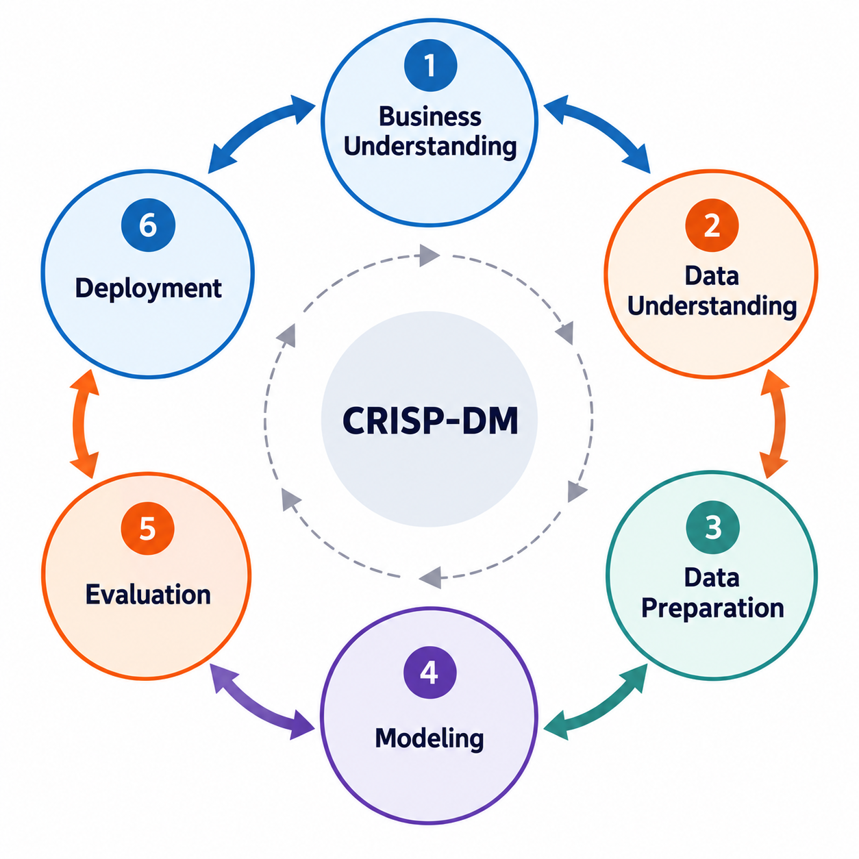
The arrows go in both directions. You rarely go through the stages once: what you find in one stage often sends you back to an earlier one. Each section of this notebook is one stage, and the diagram at the top of each section marks where you are.
The project is small on purpose, so that you can see the whole process at once. The next two modules go deeper into the stages: Data Preparation and Data Understanding in Module 2, and Modeling & Evaluation at the start of Module 3.
Outline
- Business Understanding
- Data Understanding
- Data Preparation
- Modeling
- Evaluation
- Deployment
- The stages in more depth
1. Business Understanding
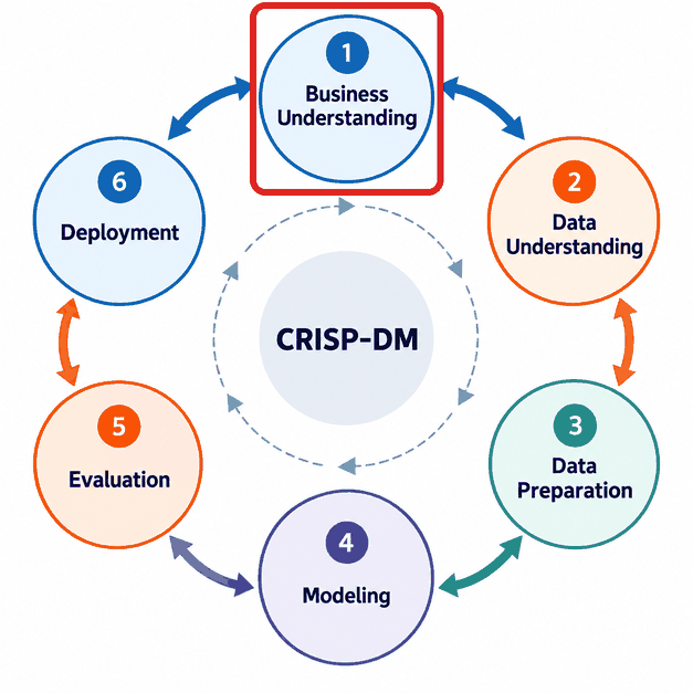
A project starts with the problem that the model should help to solve. The data in this notebook is real: the Palmer penguins dataset from Getting Started, with measurements of 344 penguins of three species (Adelie, Chinstrap and Gentoo) on three islands in Antarctica, collected by Dr. Kristen Gorman and the Palmer Station Long Term Ecological Research program. The project around it is made up for this notebook.
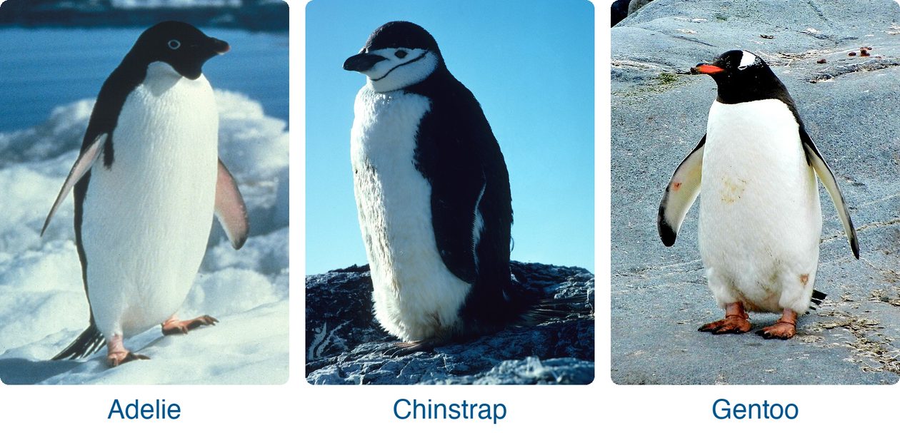
Adelie: NOAA NMFS SWFSC Antarctic Marine Living Resources (AMLR) Program, Wikimedia Commons, public domain. Chinstrap: Dr. Wayne Trivelpiece, NOAA, Wikimedia Commons, public domain. Gentoo: Jay Ruzesky, Unsplash via Wikimedia Commons, CC0.
A team of ecologists counts the penguins of each species in colonies along the coast. Telling the three species apart takes an expert, and there are not enough experts to visit every colony. Volunteers can visit more colonies, and they can measure a penguin: the length of its flipper (wing), the length and depth of its culmen (the upper ridge of the bill), and its body mass.
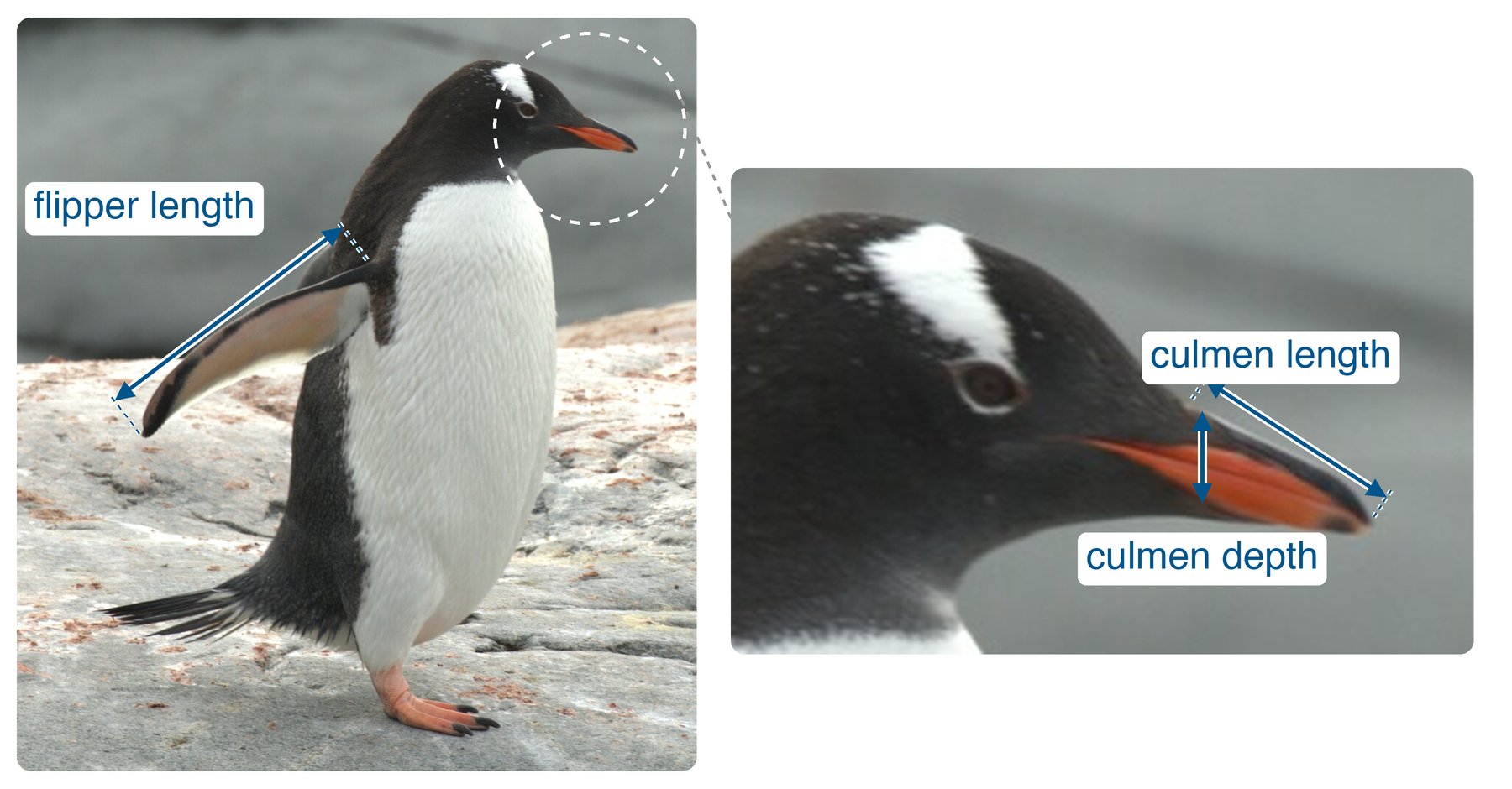
Photo: Kyle Bowman, Wikimedia Commons, CC0. Measurements added for this course.
The team asks: can a model tell the species from these four measurements, so that volunteers can do the counting?
Before you look at the data, write down the answers to a few questions together with the client:
- What should the model predict? The species of a penguin: one of three classes, so this is a classification problem.
- How will the model be used? Volunteers measure penguins in new colonies, on other islands than the ones in the data. So the model may only use what a volunteer can measure: the four measurements. It may not use the island, and it may not use the sex of the penguin, because volunteers cannot tell male and female penguins apart by looking at them.
- When is the model good enough? The team counts each species, so every species matters, also the less common ones. The team agrees on a success criterion: the model identifies at least 95% of all penguins correctly, and at least 90% of the penguins of each species.
- Which data is there? A table of 344 penguins whose species an expert identified, with the four measurements, the island and the sex.
These answers guide the rest of the project. They decide which features you may use (section 3) and how you judge the model (section 5).
2. Data Understanding
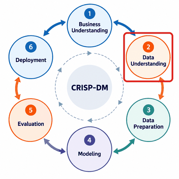
In this stage you get to know the data: what each column contains, which values are missing or wrong, and how the features relate to the target. We load the dataset from OpenML, as in the Classification notebook. frame holds the whole table as a DataFrame.
from sklearn.datasets import fetch_openml

df = fetch_openml(name="penguins", version=1, as_frame=True).frame
df.head()| species | island | culmen_length_mm | culmen_depth_mm | flipper_length_mm | body_mass_g | sex | |
|---|---|---|---|---|---|---|---|
| 0 | Adelie | Torgersen | 39.1 | 18.7 | 181.0 | 3750.0 | MALE |
| 1 | Adelie | Torgersen | 39.5 | 17.4 | 186.0 | 3800.0 | FEMALE |
| 2 | Adelie | Torgersen | 40.3 | 18.0 | 195.0 | 3250.0 | FEMALE |
| 3 | Adelie | Torgersen | NaN | NaN | NaN | NaN | NaN |
| 4 | Adelie | Torgersen | 36.7 | 19.3 | 193.0 | 3450.0 | FEMALE |
df.shape(344, 7)Each row is one penguin. species is the target, the column the model should predict.
Before we look closer, we set aside a test set. We use it only once, in section 5, to check the final model. If you study the test penguins now, what you see can influence your decisions about features and models, and then the final check is no longer a fair test on unseen data. So we explore the training set only.
stratify=df['species'] keeps the share of each species the same in both sets.
from sklearn.model_selection import train_test_split

train_df, test_df = train_test_split(df, test_size=0.2, random_state=0, stratify=df['species'])
train_df.shape, test_df.shape
((275, 7), (69, 7))First, the missing values in each column:
train_df.isna().sum()species 0
island 0
culmen_length_mm 1
culmen_depth_mm 1
flipper_length_mm 1
body_mass_g 1
sex 7
dtype: int64One penguin has no measurements at all, and seven have no value for sex. Let’s look at the values of sex:
train_df['sex'].value_counts(dropna=False)sex
FEMALE 139
MALE 128
NaN 7
_ 1
Name: count, dtype: int64Next to MALE, FEMALE and the missing values (NaN), one penguin has the value _. That is probably a typing error. In a real project you would ask the team what it means. Here it does not matter, because the model will not use sex.
How many penguins of each species are there?
train_df['species'].value_counts()species
Adelie 122
Gentoo 99
Chinstrap 54
Name: count, dtype: int64Chinstrap penguins are less common than the other two species. That is one reason to check the result for each species in section 5, and not only the overall accuracy.
The mean of each measurement per species:
features = ['culmen_length_mm', 'culmen_depth_mm', 'flipper_length_mm', 'body_mass_g']

train_df.groupby('species', observed=True)[features].mean().round(1)| culmen_length_mm | culmen_depth_mm | flipper_length_mm | body_mass_g | |
|---|---|---|---|---|
| species | ||||
| Adelie | 38.7 | 18.2 | 189.9 | 3676.4 |
| Chinstrap | 48.8 | 18.4 | 195.5 | 3739.4 |
| Gentoo | 47.5 | 14.9 | 217.0 | 5050.0 |
Gentoo penguins are the heaviest, with the longest flippers and the shallowest culmen. Adelie penguins have a much shorter culmen than the other two species. Chinstrap penguins have a long culmen, like Gentoo, but a deep one, like Adelie.
A plot shows whether the species also differ for individual penguins, and not only on average:
plt.figure(dpi=100)
for species, marker in zip(['Adelie', 'Chinstrap', 'Gentoo'], ['o', 's', '^']):
    group = train_df[train_df['species'] == species]
    plt.scatter(group['culmen_length_mm'], group['culmen_depth_mm'], marker=marker, alpha=0.7, label=species)
plt.xlabel('culmen length (mm)')
plt.ylabel('culmen depth (mm)')
plt.legend()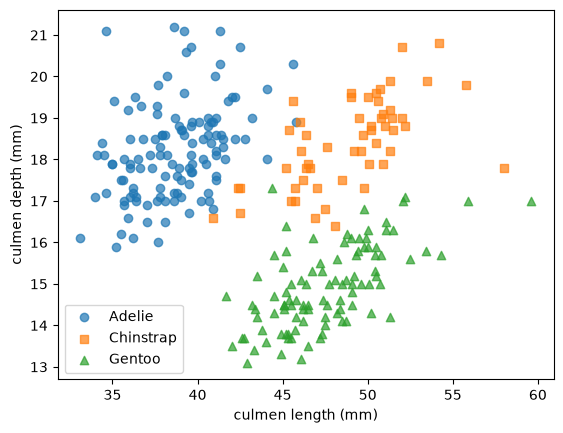
With only two of the four measurements, the three species already form three groups that hardly overlap. That is a good sign: the measurements carry the information the model needs.
Finally, the islands:
pd.crosstab(train_df['species'], train_df['island'])| island | Biscoe | Dream | Torgersen |
|---|---|---|---|
| species | |||
| Adelie | 37 | 44 | 41 |
| Chinstrap | 0 | 54 | 0 |
| Gentoo | 99 | 0 | 0 |
In this data, Gentoo penguins live only on Biscoe and Chinstrap penguins only on Dream. A model that is allowed to use island would learn these shortcuts and look very good on this data. In a new colony on another island they are useless. This confirms the decision from section 1 to leave the island out.
3. Data Preparation
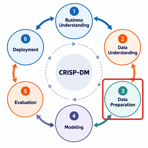
In this stage you turn the raw table into the inputs X and the target y that a model can learn from. Here that takes two decisions:
- Features: the four measurements, as decided in section 1.
- Missing values: two penguins in the whole dataset have no measurements, one in the training set and one in the test set. A model cannot predict anything for a penguin without measurements, so we remove these two rows from both sets. When only some values of a row are missing, you can often fill them in instead; the Data Preparation notebook shows how.
We apply the same steps to the training set and to the test set.
train_clean = train_df.dropna(subset=features)
test_clean = test_df.dropna(subset=features)

X_train, y_train = train_clean[features], train_clean['species']
X_test, y_test = test_clean[features], test_clean['species']

X_train.shape, X_test.shape
((274, 4), (68, 4))Many projects need more preparation than this. Models such as support vector machines need features on similar scales, and text columns such as island must be turned into numbers before a model can use them. We use a random forest, which does not need scaled features, and no text columns, so neither step is needed here. The Data Preparation notebook covers both.
4. Modeling
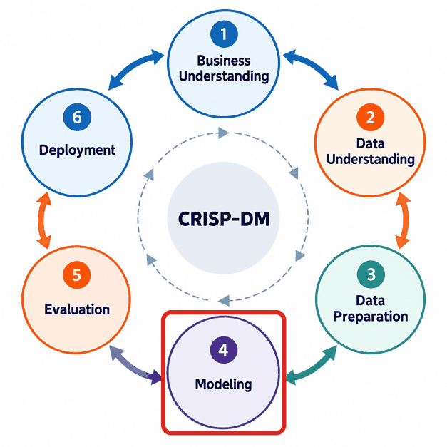
In this stage you train models. Start with a baseline, as in the Regression notebook: a “model” that ignores the features. For classification, the simplest baseline always predicts the most common class of the training set. scikit-learn has it as DummyClassifier. Any real model must do better than this.
from sklearn.dummy import DummyClassifier

baseline = DummyClassifier(strategy='most_frequent')
baseline.fit(X_train, y_train)DummyClassifier(strategy='most_frequent')In a Jupyter environment, please rerun this cell to show the HTML representation or trust the notebook.
On GitHub, the HTML representation is unable to render, please try loading this page with nbviewer.org.
Parameters
Fitted attributes
Now a random forest, the model from the Classification notebook, with its default hyperparameters. Hyperparameters are the settings you choose before training, such as the number of trees, like the degree on the What is Machine Learning? page; training does not change them:
from sklearn.ensemble import RandomForestClassifier

model = RandomForestClassifier(random_state=0)
model.fit(X_train, y_train)RandomForestClassifier(random_state=0)In a Jupyter environment, please rerun this cell to show the HTML representation or trust the notebook.
On GitHub, the HTML representation is unable to render, please try loading this page with nbviewer.org.
Parameters
Fitted attributes
In a larger project you would try several models and hyperparameters in this stage, and compare them without using the test set. The Modeling & Evaluation notebook shows how. Here we keep the first model and move on.
5. Evaluation
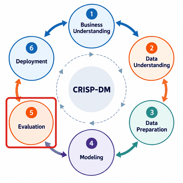
In this stage you check whether the model meets the success criterion from section 1. Now, and only now, we use the test set.
from sklearn.metrics import accuracy_score

y_pred = model.predict(X_test)

print(f"baseline accuracy:      {accuracy_score(y_test, baseline.predict(X_test)):.3f}")
print(f"random forest accuracy: {accuracy_score(y_test, y_pred):.3f}")
baseline accuracy: 0.441
random forest accuracy: 0.985The baseline predicts Adelie for every penguin and gets 44% right, the share of Adelie penguins in the test set. The random forest is far better. The success criterion also asks for every species, so we check the share of correct predictions per species, and the confusion matrix, which shows the true species in the rows and the predicted species in the columns.
from sklearn.metrics import ConfusionMatrixDisplay

results = pd.DataFrame({'species': y_test, 'correct': y_test == y_pred})
print(results.groupby('species', observed=True)['correct'].mean().round(3))

ConfusionMatrixDisplay.from_predictions(y_test, y_pred)
species
Adelie 0.967
Chinstrap 1.000
Gentoo 1.000
Name: correct, dtype: float64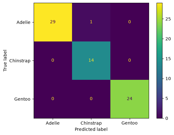
The model identifies about 98.5% of the test penguins correctly, and at least 96.7% of each species. Both parts of the success criterion are met.
Two cautions. First, the test set has only 68 penguins, so one mistake changes the accuracy by 1.5 percentage points. With another split, the numbers would be a bit different. The Modeling & Evaluation notebook shows cross-validation, which gives a more reliable estimate. Second, a good score is not the end of evaluation. Look at the mistakes too:
test_clean[y_test != y_pred]| species | island | culmen_length_mm | culmen_depth_mm | flipper_length_mm | body_mass_g | sex | |
|---|---|---|---|---|---|---|---|
| 19 | Adelie | Torgersen | 46.0 | 21.5 | 194.0 | 4200.0 | MALE |
The only mistake is an Adelie penguin with a culmen of 46 mm, which the model takes for a Chinstrap. Adelie penguins have a culmen of 38.7 mm on average, and Chinstrap penguins 48.8 mm (see section 2), so this is an unusual Adelie, closer to a Chinstrap. Mistakes like this one are hard to avoid with these four measurements.
Before the decision, check that the test set matches how the model will be used. The volunteers will measure penguins on other islands, but the test penguins come from the same three islands as the training penguins. The test score estimates how well the model does on new penguins from these islands; on a new island it can do worse, for example if the penguins there are larger or smaller. With this dataset we cannot test that: Chinstrap penguins live only on Dream and Gentoo penguins only on Biscoe, so a model trained without one of these islands never sees one of the species. Leakage & Distribution Shift in Module 2 shows how much the score can drop on another island, and Modeling & Evaluation in Module 3 shows how to validate on an island the model has not seen.
The evaluation ends with a decision. The model meets the success criterion on these three islands, so we deploy it, and an expert checks a sample of its predictions on the first new island. If it had not met the criterion, the arrows in the diagram show where to go next: back to Modeling to try other models, back to Data Preparation or Data Understanding, or even back to Business Understanding, to agree on another goal or to collect other data.
6. Deployment
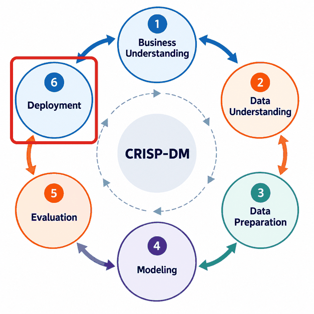
In this stage the model is put to use. For the penguin team, that could be a phone app in which a volunteer types in the four measurements and sees the predicted species. The first step is always the same: save the trained model to a file, so that other programs can load it without training it again. joblib saves and loads Python objects such as models. We save the model in the models/ folder of the course repository.
import joblib
from pathlib import Path

Path('../../../models').mkdir(exist_ok=True) # create the folder if it does not exist
joblib.dump(model, '../../../models/penguin_species.joblib')['../../../models/penguin_species.joblib']The app loads the model and predicts the species of two penguins that a volunteer has just measured. predict_proba gives the probability of each species, in the order of classes_:
loaded_model = joblib.load('../../../models/penguin_species.joblib')

new_penguins = pd.DataFrame({
    'culmen_length_mm': [50.5, 44.0],
    'culmen_depth_mm': [15.6, 18.5],
    'flipper_length_mm': [222.0, 193.0],
    'body_mass_g': [5500.0, 3800.0],
})

predictions = pd.DataFrame(loaded_model.predict_proba(new_penguins).round(2), columns=loaded_model.classes_)
predictions['predicted species'] = loaded_model.predict(new_penguins)
predictions| Adelie | Chinstrap | Gentoo | predicted species | |
|---|---|---|---|---|
| 0 | 0.00 | 0.00 | 1.00 | Gentoo |
| 1 | 0.44 | 0.55 | 0.01 | Chinstrap |
The model is sure about the first penguin: a heavy penguin with long flippers and a shallow culmen is a Gentoo. About the second penguin it is unsure: it predicts Chinstrap, but gives Adelie almost the same probability. An app can use this, for example by asking the volunteer to take a photo for an expert whenever the highest probability is low.
Deployment does not end when the model is in use. The team should keep checking it, for example by asking an expert to identify a sample of the penguins in each new colony and comparing with the model. Penguins in a new colony can differ from the ones in the training data, for example because there is more or less food there, and then the model can make more mistakes than in section 5. When that happens, the team collects new data and trains the model again. Deployment can even show that the problem was defined wrongly, for example if volunteers cannot measure body mass in the field. Then the project goes back to Business Understanding.
You have now been through all six stages once. In a real project you go through them many times, and each time you know more about the problem and the data.
7. The stages in more depth
Modules 2 and 3 of the Self-study go deeper into the stages:
- Data Preparation (Module 2): scaling, transforming skewed features, missing values, merging and encoding.
- Data Understanding (Module 2): the distribution of each feature, relationships between features, and PCA.
- Modeling & Evaluation (Module 3): cross-validation, validation and test sets, feature and model selection, hyperparameter tuning, and evaluation metrics.
Data Preparation comes before Data Understanding in this list, the other way around from CRISP-DM. That is on purpose. To understand a dataset, you often have to prepare it first. You scale features before you compare them, transform a skewed feature before you can see its shape, and turn text columns into numbers before you can compute correlations with them. So the work in the Data Understanding stage already uses data preparation, and the Data Preparation notebook gives you those tools first. In a project, you still follow the CRISP-DM order, and you move back and forth between the two stages.
Further reading (optional)
- Aurélien Géron, Hands-On Machine Learning with Scikit-Learn, Keras & TensorFlow (O’Reilly), chapter 2, “End-to-End Machine Learning Project”: a larger project on California house prices, with the same stages.