# Installs the missing packages on Google Colab only; does nothing locally.
import sys

if "google.colab" in sys.modules:
%pip install -q optunaModeling and Evaluation

This notebook is worth revisiting more than once: each time, you will notice something new. It contains 3 parts with each part containing 3 sections. The notebook concludes with the exercises.
- Part 1: Model Evaluation
- Cross-Validation
- Train/Validation/Test Split
- Train/Validation/Test Split and Cross-Validation
- Part 2: Improving Model Performance
- Feature Selection and Engineering
- Model Selection
- Hyperparameter Tuning
- Part 3: Model Evaluation (yes, again)
- Underfitting and Overfitting
- Evaluating Classification Models
- Evaluating Regression Models
- Exercises
Working in Colab? This notebook uses optuna, which Colab does not include. Run the cell below: it installs the package only when it detects Colab. Locally it does nothing, because the course environment already includes optuna.
import numpy as np
import pandas as pd
import matplotlib.pyplot as plt

from sklearn.datasets import fetch_openml, load_diabetes, fetch_california_housing, load_breast_cancer
Part 1: Model Evaluation
In this part, we explore how to evaluate models reliably. You’ll learn the key ideas behind train/validation/test splits and cross-validation, and understand why a single train/test split can give misleading results. By the end of this part, you’ll know how to design proper evaluation procedures that give trustworthy estimates of model performance.
1. Cross-Validation
In the Classification and Regression notebooks, we evaluated our models using a simple train/test split. However, you may have noticed that the results vary depending on how the data is split. For example in classification, one split might give an accuracy of 0.94, while another gives 0.96. So which result should we use for downstream decisions such as model selection or deployment? Or should we instead report an average, such as 0.95?
from sklearn.ensemble import RandomForestClassifier
from sklearn.metrics import accuracy_score
from sklearn.model_selection import train_test_split
X, y = load_breast_cancer(as_frame=True, return_X_y=True)# split with random_state=0
X_train, X_test, y_train, y_test = train_test_split(X, y, test_size=0.2, random_state=0)
model = RandomForestClassifier(random_state=0)
model.fit(X_train, y_train)
y_pred = model.predict(X_test)
accuracy = accuracy_score(y_test, y_pred)
print(accuracy)0.9649122807017544# split with random_state=1
X_train, X_test, y_train, y_test = train_test_split(X, y, test_size=0.2, random_state=1)
model = RandomForestClassifier(random_state=0)
model.fit(X_train, y_train)
y_pred = model.predict(X_test)
accuracy = accuracy_score(y_test, y_pred)
print(accuracy)0.9473684210526315What if we use a for loop to vary the random state from 0 to 99 and record the results each time?
accuracy_results = []
for random_state in range(100):
    X_train, X_test, y_train, y_test = train_test_split(X, y, test_size=0.2, random_state=random_state)
    model = RandomForestClassifier(random_state=0)
    model.fit(X_train, y_train)
    y_pred = model.predict(X_test)
    accuracy = accuracy_score(y_test, y_pred)
accuracy_results.append(accuracy)min(accuracy_results), max(accuracy_results)
print(f"Min accuracy: {min(accuracy_results):.4f}")
print(f"Avg accuracy: {sum(accuracy_results)/len(accuracy_results):.4f}")
print(f"Max accuracy: {max(accuracy_results):.4f}")Min accuracy: 0.9035
Avg accuracy: 0.9589
Max accuracy: 0.9912In my case, the accuracy ranged from 0.9035 to 0.9912, with an average of 0.9589. You might get different results, but you will still notice a significant variation. Note that we only changed how we split the data, yet the results vary by almost 9 percentage points. This variation happens due to random fluctuations in how the data is sampled.
Statistics courses explore this concept in depth, but for now, you just need to know that sampling is the process of selecting a subset of data points from a larger population, and the variation we observe is called sampling error.
Also remember, our ultimate goal is not to measure accuracy on the current test set, it’s to estimate how accurately the model will perform on unseen, future data.
Let’s now check the distribution of the accuracy scores:
plt.hist(accuracy_results)(array([ 2., 0., 2., 3., 27., 0., 15., 18., 17., 16.]),
array([0.90350877, 0.9122807 , 0.92105263, 0.92982456, 0.93859649,
0.94736842, 0.95614035, 0.96491228, 0.97368421, 0.98245614,
0.99122807]),
<BarContainer object of 10 artists>)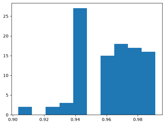
Our best estimate for the model’s accuracy on unseen data is 0.9589. However, obtaining this estimate required training the model 100 times, which is quite inefficient. Instead, we can systematically split the data into subsets and train/test in a way that ensures each sample is used for both training and testing at least once.
Imagine we split the dataset into 5 equal blocks (called folds). Each fold is used once as the test set, and the remaining blocks form the training set. Indices 1–10 are just placeholders to show order.
Test set · Training set
Fold 1: [1, 2, 3, 4, 5, 6, 7, 8, 9, 10]
Fold 2: [1, 2, 3, 4, 5, 6, 7, 8, 9, 10]
Fold 3: [1, 2, 3, 4, 5, 6, 7, 8, 9, 10]
Fold 4: [1, 2, 3, 4, 5, 6, 7, 8, 9, 10]
Fold 5: [1, 2, 3, 4, 5, 6, 7, 8, 9, 10]
This approach is called 5-fold cross-validation. In general this is called k-fold cross validation where k is the number of folds. For example 10-fold cross validation would look like this:
Fold 1: [1, 2, 3, 4, 5, 6, 7, 8, 9, 10]
Fold 2: [1, 2, 3, 4, 5, 6, 7, 8, 9, 10]
…
Fold 10: [1, 2, 3, 4, 5, 6, 7, 8, 9, 10]
scikit learn has multiple ways to implement cross-validation
from sklearn.model_selection import KFold
kf = KFold(n_splits=5, shuffle=False)
the kf above is a K-fold cross-validation splitter that will divide your dataset into 5 sequential folds, without shuffling the data first.
dummy_x = np.array([1, 2, 3, 4, 5, 6, 7, 8, 9, 10])fold_id = 1
for train_indices, test_indices in kf.split(dummy_x):
print(f"---Fold {fold_id}---")
print("Test Set:", dummy_x[test_indices])
print("Training Set:", dummy_x[train_indices])
fold_id += 1---Fold 1---
Test Set: [1 2]
Training Set: [ 3 4 5 6 7 8 9 10]
---Fold 2---
Test Set: [3 4]
Training Set: [ 1 2 5 6 7 8 9 10]
---Fold 3---
Test Set: [5 6]
Training Set: [ 1 2 3 4 7 8 9 10]
---Fold 4---
Test Set: [7 8]
Training Set: [ 1 2 3 4 5 6 9 10]
---Fold 5---
Test Set: [ 9 10]
Training Set: [1 2 3 4 5 6 7 8]now let’s apply this idea to the actual dataset:
# easier to slice numpy arrays
X = np.array(X)
y = np.array(y)
accuracy_results = []
for train_indices, test_indices in kf.split(X):
# instead of train/test split randomly
# we use the indices coming from k-fold cv
X_train = X[train_indices]
y_train = y[train_indices]
X_test = X[test_indices]
y_test = y[test_indices]
# this part is the same
model = RandomForestClassifier(random_state=0)
model.fit(X_train, y_train)
y_pred = model.predict(X_test)
accuracy = accuracy_score(y_test, y_pred)
accuracy_results.append(accuracy)print(f"Avg accuracy: {sum(accuracy_results)/len(accuracy_results):.4f}")Avg accuracy: 0.9614This time, with only 5 training runs (instead of 100), we obtained a very similar accuracy estimate. We can do this without an explicit for loop using cross_validate and providing kf as a parameter.
from sklearn.model_selection import cross_validate
cv_results = cross_validate(model, X, y, cv=kf)cv_results{'fit_time': array([0.07070494, 0.06901121, 0.06970811, 0.07084799, 0.08113503]),
'score_time': array([0.00315404, 0.0031538 , 0.00311399, 0.00309777, 0.003232 ]),
'test_score': array([0.92982456, 0.95614035, 0.98245614, 0.96491228, 0.97345133])}np.mean(cv_results['test_score'])np.float64(0.9613569321533924)note that this is doing exactly the same thing we did with the for loop above.
cv_results = cross_validate(model, X, y, cv=10) # cv parameter can also work with an integer directly
np.mean(cv_results['test_score'])np.float64(0.9649122807017545)Cross-validation for classification: stratified folds. KFold(shuffle=False) above cuts the data into consecutive blocks. That is fine to show the idea, but if a dataset happens to be sorted by class, some folds get few or none of one class. For classification, use StratifiedKFold: it keeps the class proportions of y roughly the same in every fold (you will see stratification again in section 8). Shuffle with a fixed random_state, so that your results are reproducible.
This also explains the last cell: when you pass an integer such as cv=10 with a classifier, scikit-learn uses StratifiedKFold (without shuffling), not KFold, so its result can differ from the explicit KFold above. For regression, KFold is the usual choice.
Whatever you choose, give every model you compare the same cv object and metric. Otherwise a difference in scores may come from different folds, not from a better model.
from sklearn.model_selection import StratifiedKFold
skf = StratifiedKFold(n_splits=5, shuffle=True, random_state=0)
cv_results = cross_validate(model, X, y, cv=skf)
np.mean(cv_results['test_score'])np.float64(0.9648812296227295)2. Train/Validation/Test Split
In the End-to-End ML Project notebook, the test set was set aside at the very beginning and used only once, at the very end. During model development, however, we often need to test many ideas. For example, when comparing two different algorithms, how do we decide which one performs better? In this section, you’ll look at this problem more closely.
In the previous section we have solved the sampling error problem that occurs with a single train/test split by using cross-validation. However, one issue still remains.
In practice, model development involves trying out different ideas such as testing new models, changing hyperparameters, or adding features, and checking the cross-validation score to see if things improved. But if we keep doing this repeatedly, we start optimizing for this particular dataset, which leads to a subtle form of overfitting.
To prevent this, we need a truly independent dataset that the model has never influenced in any way. This is where the test set comes in. The test set should be used only once, at the very end of the process. The moment you look at the test results and use them to guide improvements, you are unintentionally leaking information from the test data into the model.
To handle this correctly, we create three datasets instead of just one split:
- Training set used to fit the model
- Validation set used during development to tune and compare models
- Test set used only once at the end to estimate the performance on new data
The workflow looks like this:
- First, split the data into a Development set and a Test set.
- Then, split the Development set again into Training and Validation parts.
A common ratio is 80% / 10% / 10% for Train / Validation / Test, though this can vary depending on dataset size.
This is also why machine-learning competitions, such as those on Kaggle, often have a public and a private leaderboard. The public leaderboard scores one part of the test data. You only see the score, not the data, but if you keep adjusting your model to climb higher on it, you might end up overfitting to that part. The private leaderboard scores the other part and is revealed only at the end. It shows how well your model truly generalizes to unseen data.
YOUR TURN
I think you know enough to do this without me showing it first. The solution will be provided below, please try first without LLMs or looking at my solution. Then compare your solution with mine.
X, y = load_breast_cancer(as_frame=True, return_X_y=True)Use train_test_split and split the dataset into train/val/test. (Hint: use it twice)
print(f"Create a training set (X_train, y_train) with 80% of the dataset, which corresponds to {X.shape[0] * 0.8:.0f} data points")
print(f"Create a validation set (X_val, y_val) with 10% of the dataset, which corresponds to {X.shape[0] * 0.1:.0f} data points")
print(f"Create a test set (X_test, y_test) with 10% of the dataset, which corresponds to {X.shape[0] * 0.1:.0f} data points")
Create a training set (X_train, y_train) with 80% of the dataset, which corresponds to 455 data points
Create a validation set (X_val, y_val) with 10% of the dataset, which corresponds to 57 data points
Create a test set (X_test, y_test) with 10% of the dataset, which corresponds to 57 data points# YOUR CODE HERE# Verify the results
try:
assert(X_train.shape[0] == 455)
assert(X_val.shape[0] == 57)
assert(X_test.shape[0] == 57)
print("Looks like it is working!")
except Exception as e:
print(e)Here is my solution:
First, split the data into a Development set (9/10) and a Test set (1/10).
Then, split the Development set again into Training and Validation (careful: 1/10 of the whole set but 1/9 of the development set) parts.
# My solution
X_dev, X_test, y_dev, y_test = train_test_split(X, y, test_size=1/10, random_state=0)
X_train, X_val, y_train, y_val = train_test_split(X_dev, y_dev, test_size=1/9, random_state=0)
X_train.shape, X_val.shape, X_test.shape((455, 30), (57, 30), (57, 30))So now the process becomes:
- Do the development with the development set (X_train, y_train) and (X_val, y_val)
- Decide on the final model based on the validation performance.
- Retrain the final model on the development set (X_dev, y_dev) (think a little why this is the case)
- Use (X_test, y_test) only once to estimate the performance
Typically step 1 takes a lot of time. But for demonstration purposes, imagine step 1 only consists of deciding which one is better RandomForestClassifier or DecisionTreeClassifier.
# STEP 1 Do the development with the development set (X_train, y_train) and (X_val, y_val)
# load and split

X, y = load_breast_cancer(as_frame=True, return_X_y=True)
X_dev, X_test, y_dev, y_test = train_test_split(X, y, test_size=1/10, random_state=0)
X_train, X_val, y_train, y_val = train_test_split(X_dev, y_dev, test_size=1/9, random_state=0)
X_train.shape, X_val.shape, X_test.shape
((455, 30), (57, 30), (57, 30))# STEP 1 Do the development with the development set (X_train, y_train) and (X_val, y_val)
# call both models
from sklearn.ensemble import RandomForestClassifier
from sklearn.tree import DecisionTreeClassifier
model_rfc = RandomForestClassifier(random_state=0)
model_dtc = DecisionTreeClassifier(random_state=0)# STEP 1 Do the development with the development set (X_train, y_train) and (X_val, y_val)
# train/validate random forest
model_rfc.fit(X_train, y_train)
y_pred = model_rfc.predict(X_val)
accuracy = accuracy_score(y_val, y_pred)
print(accuracy)0.9824561403508771# STEP 1 Do the development with the development set (X_train, y_train) and (X_val, y_val)
# train/validate decision tree
model_dtc.fit(X_train, y_train)
y_pred = model_dtc.predict(X_val)
accuracy = accuracy_score(y_val, y_pred)
print(accuracy)0.9298245614035088STEP 2: Decide on the final model based on the validation performance.
I obtained random forest (0.98) > decision tree (0.93) so I decided RandomForestClassifier is better.
# STEP 3 Retrain the final model on the development set (X_dev, y_dev)

model_rfc = RandomForestClassifier(random_state=0)
model_rfc.fit(X_dev, y_dev) # instead of X_train, y_trainRandomForestClassifier(random_state=0)In a Jupyter environment, please rerun this cell to show the HTML representation or trust the notebook.
On GitHub, the HTML representation is unable to render, please try loading this page with nbviewer.org.
Parameters
Fitted attributes
# STEP 4 Use (X_test, y_test) only once to estimate the performance
y_pred = model_rfc.predict(X_test) # instead of X_val
accuracy = accuracy_score(y_test, y_pred) # instead of y_val
print(accuracy)0.9298245614035088Now you might have noticed that splitting the data into train/val/test doesn’t remove the need for cross-validation. How should we combine the two?
3. Train/Val/Test Split and Cross-Validation
Scikit-learn has a guide with the following image that explains how to combine these two concepts.
https://scikit-learn.org/stable/modules/cross_validation.html
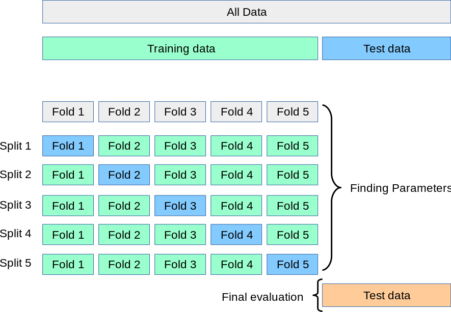
The image shows how cross-validation can be combined with the train/validation/test split concept. First, divide the dataset into two parts: a development set (called training data in the image) and a test set. Next, apply cross-validation within the development set to tune and compare models. Once the best model is selected, retrain it on the full development set and finally evaluate it on the test set to estimate how well it performs on new data. With 57 test samples this estimate is still rough: its standard error is about 3 percentage points of accuracy.
Let’s update our process accordingly:
- Do the development with the development set and cross-validation
- Decide on the final model based on the cross-validation performance
- Retrain the final model on the development set (X_dev, y_dev)
- Use (X_test, y_test) only once to estimate the performance
# STEP 1 Do the development with the development set and cross-validation
# load and split

X, y = load_breast_cancer(as_frame=True, return_X_y=True)
X_dev, X_test, y_dev, y_test = train_test_split(X, y, test_size=1/10, random_state=0)
# STEP 1 Do the development with the development set and cross-validation
# call models
from sklearn.ensemble import RandomForestClassifier
from sklearn.tree import DecisionTreeClassifier
model_rfc = RandomForestClassifier(random_state=0)
model_dtc = DecisionTreeClassifier(random_state=0)# STEP 1 Do the development with the development set and cross-validation
# cross validate random forest
from sklearn.model_selection import StratifiedKFold
from sklearn.model_selection import cross_validate
# stratified and shuffled folds, as recommended in section 1
skf = StratifiedKFold(n_splits=5, shuffle=True, random_state=0)
cv_results = cross_validate(model_rfc, X_dev, y_dev, cv=skf)
np.mean(cv_results['test_score'])np.float64(0.9589948600799543)# STEP 1 Do the development with the development set and cross-validation
# cross validate decision tree
# the same folds for both models
cv_results = cross_validate(model_dtc, X_dev, y_dev, cv=skf)
np.mean(cv_results['test_score'])np.float64(0.9335808109651629)STEP 2: Decide on the final model based on the cross-validation performance
I obtained random forest (0.96) > decision tree (0.93) so I decided RandomForestClassifier is better.
# STEP 3
# Retrain the final model on the development set (X_dev, y_dev)

model_rfc = RandomForestClassifier(random_state=0)
model_rfc.fit(X_dev, y_dev) # instead of X_train, y_trainRandomForestClassifier(random_state=0)In a Jupyter environment, please rerun this cell to show the HTML representation or trust the notebook.
On GitHub, the HTML representation is unable to render, please try loading this page with nbviewer.org.
Parameters
Fitted attributes
# STEP 4
# Use (X_test, y_test) only once to estimate the performance
y_pred = model_rfc.predict(X_test) # instead of X_val
accuracy = accuracy_score(y_test, y_pred) # instead of y_val
print(accuracy)0.9298245614035088YOUR TURN
I got the same test accuracy. If the result is the same as using a simple train/validation/test split, why go through the extra step of cross-validation? Or, put differently: in what situations is cross-validation on the development set more beneficial than a single train/validation/test split?
# YOUR ANSWER HEREOne possible answer
Here both procedures chose the random forest, so the test accuracy is the same. They can disagree when the difference between two models is small or the validation set is small. A validation set of 57 samples gives a noisy score: another split could have favored the other model. Cross-validation uses every sample of the development set for validation once, so the comparison rests on 512 samples instead of 57, and the spread over the folds shows how much the score varies. It costs more training time, which is why a single validation set is used when the data or the models are large.
Cross-validation by group
KFold and StratifiedKFold put the samples into folds at random. The cross-validation score then estimates how well the model predicts new samples like the ones it was trained on. Often a model is used on data that comes from somewhere else: another hospital, another machine, another island. Then the validation folds should come from somewhere else as well.
The penguins from the End-to-End ML Project notebook were measured on three islands. Suppose we want to predict the body mass of a penguin from its bill and flipper measurements, and the model will be used for penguins on other islands. We compare random folds with folds by island.
penguins = fetch_openml(name="penguins", version=1, as_frame=True).frame
measurements = ['culmen_length_mm', 'culmen_depth_mm', 'flipper_length_mm']
penguins = penguins.dropna(subset=measurements + ['body_mass_g']).reset_index(drop=True)

X_penguins = penguins[measurements]
y_penguins = penguins['body_mass_g']
islands = penguins['island']
islands.value_counts()
island
Biscoe 167
Dream 124
Torgersen 51
Name: count, dtype: int64With random folds:
from sklearn.ensemble import RandomForestRegressor

model = RandomForestRegressor(random_state=0)
kf = KFold(n_splits=5, shuffle=True, random_state=0)
cv_results = cross_validate(model, X_penguins, y_penguins, cv=kf, scoring='neg_mean_absolute_error')
print(f"MAE with random folds: {-cv_results['test_score'].mean():.0f} g")
MAE with random folds: 276 gGroupKFold keeps all samples of a group in the same fold. You pass the group of every sample with groups=. With three islands and n_splits=3, every fold is one island: the model is trained on two islands and validated on the third.
from sklearn.model_selection import GroupKFold

gkf = GroupKFold(n_splits=3)
cv_results = cross_validate(model, X_penguins, y_penguins, cv=gkf, groups=islands, scoring='neg_mean_absolute_error')
print(f"MAE with folds by island: {-cv_results['test_score'].mean():.0f} g")

for (train_idx, val_idx), score in zip(gkf.split(X_penguins, y_penguins, groups=islands), cv_results['test_score']):
    print(f"  validated on {islands.iloc[val_idx[0]]}: MAE {-score:.0f} g")
MAE with folds by island: 712 g
validated on Biscoe: MAE 1244 g
validated on Dream: MAE 589 g
validated on Torgersen: MAE 303 gThe error with folds by island is more than twice as large, and the fold that validates on Biscoe is by far the worst. In this data, Gentoo penguins, the largest of the three species, live only on Biscoe. Trained on the other two islands, the model has never seen a penguin that large, and a random forest cannot predict values outside the range of the targets it was trained on. With random folds this does not show, because every training part contains Gentoo penguins.
The two scores estimate different things: the random folds the error for new penguins from these three islands, the folds by island the error for penguins from an island the model has not seen. Choose the folds that match how the model will be used.
Sometimes you want to decide yourself which samples are used for validation. Suppose the model will be used on Dream, where you have already measured some penguins, and the penguins of Biscoe and Torgersen should always be in the training data. cv also accepts a list of (training indices, validation indices) pairs, so you can build the folds yourself: here, five folds of the Dream penguins, with the other islands added to every training part.
dream = np.where(islands == 'Dream')[0]
other_islands = np.where(islands != 'Dream')[0]

splits = []
for train_part, val_part in KFold(n_splits=5, shuffle=True, random_state=0).split(dream):
    train_idx = np.concatenate([other_islands, dream[train_part]])  # the other islands are always in training
    val_idx = dream[val_part]  # validate on Dream penguins only
    splits.append((train_idx, val_idx))

cv_results = cross_validate(model, X_penguins, y_penguins, cv=splits, scoring='neg_mean_absolute_error')
print(f"MAE on Dream penguins: {-cv_results['test_score'].mean():.0f} g")
MAE on Dream penguins: 264 gOnce some Dream penguins are in the training data, the error on Dream penguins is much lower than when Dream is left out completely (589 g in the folds by island).
The indices are row positions, as in the KFold loop of section 1. A list of splits works everywhere a cv argument does: cross_val_score, GridSearchCV, RandomizedSearchCV. Give every model you compare the same list. (PredefinedSplit is another way to fix the validation samples yourself; the list of index pairs is the most flexible.)
Part 2: Improving Model Performance
In Part 1, we focused on evaluating models. This was essential because before trying to improve model performance, we need a reliable way to measure it. Now that our evaluation framework is in place, we can shift our focus to improving model performance.
Data: You can improve performance by collecting more data or improving data quality (e.g., replacing low-resolution images with higher-resolution ones). However, the quality should match the use case, if the real-world scenario involves low-quality inputs, training only on high-quality data can actually reduce performance. Data collection and quality improvement are beyond the scope of this course: first, you need a solid understanding of machine learning to appreciate how data should be collected.
Features: You can select the most useful features (this process is called feature selection) and engineer new ones by transforming or combining existing features (this process is called feature engineering).
Models: You can try different algorithms or architectures that better fit your data and problem. (this process is called model selection)
Hyperparameters: You can tune model settings to improve performance and generalization. (this process is called hyperparameter tuning)
You should improve these aspects in the listed order for two main reasons:
Dependency: Suppose you have only 100 data points and find that model A performs better than model B. After collecting more data, say 10,000 samples, a completely different model, like C, might turn out to be the best.
Impact: Hyperparameter tuning does provide real improvements, but usually small ones. That’s why it’s best to leave it for the final step.
Do this iteratively. If you already have some data and know that more will arrive in two weeks, don’t wait, start with what you have. Write your code so that you can easily rerun the process as new data comes in, following the same order of improvement. In practice, those who can test and iterate faster often build better models than those with great ideas but fewer experiments. Design your code and workflow to enable quick iteration.
4. Feature Selection and Engineering
This topic could easily be a course on its own. There is both a methodological foundation and an element of creativity involved. For example, in a disease prediction competition I once joined, the winning team created a new feature based on room codes, they calculated the distance between patient rooms and used it as a predictor. This feature turned out to be crucial because the disease was contagious, and proximity between rooms influenced infection risk.
This illustrates that feature selection and engineering is highly problem-specific. In this section, I will show you a simple and fast approach to selecting features and another one which is more reliable but slower. However, mastering this concept ultimately comes from practice across many projects, where you learn to connect domain knowledge with data representation.
If you’re interested in learning more about this topic, check out Python Feature Engineering Cookbook by Soledad Galli. It is published by Packt and is also available on the O’Reilly learning platform, which many university and public libraries give access to.
The first method we will cover is based on the feature_importances_ attribute on a trained random forest model.
YOUR TURN
Find the feature_importances_ attribute in the documentation:
https://scikit-learn.org/stable/modules/generated/sklearn.ensemble.RandomForestClassifier.html
and use it to obtain feature importances on a model you trained before. Solution will be give below.
# YOUR CODE HEREThis shows how important each feature is for the predictions made by a Random Forest model. It measures the average reduction in impurity (like Gini or entropy) caused by each feature across all trees in the forest. The values are normalized to sum to 1, meaning a higher number indicates a greater impact on the model’s decisions.
Here is my solution:
model_rfc.feature_importances_array([0.0299234 , 0.0151687 , 0.08720372, 0.04861491, 0.00609207,
0.00575877, 0.05887879, 0.08067784, 0.00421614, 0.00362227,
0.02394147, 0.00295257, 0.01618338, 0.02841103, 0.0039015 ,
0.00502775, 0.00570331, 0.00540493, 0.00588076, 0.00528317,
0.10179607, 0.01698023, 0.16528527, 0.06936744, 0.01519418,
0.01254105, 0.02981753, 0.12946293, 0.01068686, 0.00602196])# create a df with feature importances and feature names
feat_imp = pd.DataFrame({
'Feature': X_dev.columns,
'Importance': model_rfc.feature_importances_
})
# sort
feat_imp = feat_imp.sort_values(by='Importance', ascending=False)
feat_imp.head()| Feature | Importance | |
|---|---|---|
| 22 | worst perimeter | 0.165285 |
| 27 | worst concave points | 0.129463 |
| 20 | worst radius | 0.101796 |
| 2 | mean perimeter | 0.087204 |
| 7 | mean concave points | 0.080678 |
Based on this, you can perform feature selection by either keeping the top n features or removing those with importance values below a chosen threshold. However, this approach alone doesn’t prove whether a feature is truly useful, it only measures importance within one fitted model.
A more robust method is Recursive Feature Elimination with Cross-Validation (RFECV), which repeatedly fits the model on different subsets of features and evaluates performance through cross-validation to find the optimal feature set.
from sklearn.feature_selection import RFECV
model = RandomForestClassifier(random_state=0)
selector = RFECV(model, step=1, cv=5)
selector.fit(X_dev, y_dev)
RFECV(cv=5, estimator=RandomForestClassifier(random_state=0))In a Jupyter environment, please rerun this cell to show the HTML representation or trust the notebook.
On GitHub, the HTML representation is unable to render, please try loading this page with nbviewer.org.
Parameters
Fitted attributes
RandomForestClassifier(random_state=0)
Parameters
30 features
| mean radius |
| mean texture |
| mean perimeter |
| mean area |
| mean smoothness |
| mean compactness |
| mean concavity |
| mean concave points |
| mean symmetry |
| mean fractal dimension |
| radius error |
| texture error |
| perimeter error |
| area error |
| smoothness error |
| compactness error |
| concavity error |
| concave points error |
| symmetry error |
| fractal dimension error |
| worst radius |
| worst texture |
| worst perimeter |
| worst area |
| worst smoothness |
| worst compactness |
| worst concavity |
| worst concave points |
| worst symmetry |
| worst fractal dimension |
Which gives a binary output per feature whether it is selected (True) or not (False).
print(f"The dataset has {X.shape[1]} features.")The dataset has 30 features.We can check the number of selected features as follows:
selector.n_features_np.int64(30)which is equal to the total number of features, meaning all of the features are selected! You can see the selected features here, which should all be True
selector.support_array([ True, True, True, True, True, True, True, True, True,
True, True, True, True, True, True, True, True, True,
True, True, True, True, True, True, True, True, True,
True, True, True])# the mean cross-validated accuracy for each number of features
scores = selector.cv_results_['mean_test_score']
for k in [1, 2, 5, 10, 20, 30]:
print(f"{k:2d} features: {scores[k - 1]:.3f}") 1 features: 0.885
2 features: 0.914
5 features: 0.949
10 features: 0.957
20 features: 0.961
30 features: 0.965The cross-validated accuracy rises quickly with the first features and then only slowly: from 0.957 with 10 features to 0.965 with all 30, less than one percentage point. Many of the 30 features carry overlapping information (radius, perimeter and area describe the same size), so removing one costs little. RFECV picks the number of features with the highest mean score, here all 30. That does not mean that every feature is needed. On a dataset with many unhelpful features, the curve drops once they are added, and RFECV removes them.
5. Model Selection
We already explored model selection in Part 1, where we compared two models and chose the better one. In theory, you could test every model available in scikit-learn and simply pick the one with the highest score. In practice, this is not how data scientists work.
A better approach is to make informed choices.
One of the most effective ways to make informed choices is to look at what the community is already doing. Before modelling, data scientists often scan the literature to see which algorithms tend to work well for similar problems.
What does “the literature” mean?
When we say “the literature,” we mean peer-reviewed research papers, conference papers, and sometimes technical reports written by researchers and practitioners. These documents describe what people tried, what worked, and why.
You don’t need to read papers in depth at this stage, but it is very useful to search what people typically use.
Where do you find these papers?
Here are the standard places where data scientists search:
Google Scholar https://scholar.google.com This is the search engine for academic papers. Type queries like tabular data machine learning, house price prediction algorithm, material property prediction model, etc.
arXiv https://arxiv.org A repository of research papers in machine learning, computer vision, statistics, and more.
We will cover ML research in depth in the Applied ML Research module. For now, you only need to get a feeling for it.
How to search effectively
Try queries like:
- best machine learning algorithms for tabular data
- machine learning model performance tabular datasets
- house price prediction machine learning
- material property prediction regression algorithms
You don’t need to read entire papers. Look at:
- the abstract
- the list of algorithms they compared
- the results table
- what they recommend
This is enough for now.
YOUR TURN
Search the literature to find which algorithms work best on tabular data.
You should find that tree-based algorithms dominate: Random Forest, Gradient Boosting (XGBoost, LightGBM, CatBoost), etc. Keep this in mind. We will cover gradient boosting later.
# Put a link hereYOUR TURN
Pick a specific problem (e.g. house price prediction) and search the literature to see which models people use. Report:
- the algorithms they tried
- which ones performed best
# Put a link here6. Hyperparameter Tuning
In this section we use the Optuna library for tuning. scikit-learn has its own tuning tools, which you will see at the end of this section, but they get slow for larger searches. Optuna is more efficient and easy to use, so it is worth learning from the start, even as you’re just beginning with machine learning.
Until now, we have trained our models with the default values of their hyperparameters: the settings you choose before training, such as the number of trees, as opposed to the parameters that training learns. The default values are chosen by the scikit-learn developers to work reasonably well for many problems. You can find them listed in the documentation, for example:
class sklearn.ensemble.RandomForestClassifier(n_estimators=100, *, criterion='gini', max_depth=None, min_samples_split=2, min_samples_leaf=1, min_weight_fraction_leaf=0.0, max_features='sqrt', max_leaf_nodes=None, min_impurity_decrease=0.0, bootstrap=True, oob_score=False, n_jobs=None, random_state=None, verbose=0, warm_start=False, class_weight=None, ccp_alpha=0.0, max_samples=None, monotonic_cst=None)These defaults are meant to perform reasonably well out of the box, but tuning them for your specific problem often improves performance. Not always: sometimes the defaults are already about as good as it gets (Module 4 shows an example).
One challenge with hyperparameter tuning is that it requires understanding what each parameter does. Looking at the list above, it is not easy to guess their meaning without knowing how the algorithm works. For instance, once you know that a random forest is an ensemble of decision trees, it becomes clear that n_estimators=100 means the forest has 100 trees. Reducing it to 10 makes training faster, but the average of so few trees is noisier. Increasing it to 1000 usually makes the predictions a little more stable, with gains that level off, while training and prediction get slower and the model gets larger. Adding trees does not make a random forest overfit; how complex each tree is does, which is what max_depth controls.
As you learn more about how algorithms work in this course and beyond, always connect that understanding to their hyperparameters. For example, max_depth controls how deep the trees can grow. If you fit a random forest to millions of data points with max_depth=None, the model can become several gigabytes in size. Even if performance improves slightly, it may not be practical.
Learning hyperparameter tuning takes time and experience. For now, whenever you encounter a new algorithm, try to understand a few key parameters. If you are not sure where to start, you can ask an LLM of your choice which parameters matter most and what reasonable ranges to explore.
import optunaLet’s start with a simple optimization problem in Optuna.
Which value of \(x\) gives the minimum for \((x - 2)^2\). Using your math knowledge you can solve this analytically and find \(x=2\) gives the minimum value of this function. Let’s solve this problem with Optuna numerically (meaning testing different values for x and checking the output)
# The objective function defines what we want to minimize or maximize.
# Optuna will call this function many times with different parameter values.
def objective(trial):
    x = trial.suggest_float('x', -10, 10) # Suggest a value for x between -10 and 10
    return (x - 2) ** 2 # The smaller this value, the better.
# A Study is an optimization session. It stores all trials and their results.
study = optuna.create_study()[I 2026-11-14 12:58:05,967] A new study created in memory with name: no-name-8fabf168-4449-4df3-923e-ec572d03c923
# Run the optimization process.
# Optuna will try 100 different x values, guided by past results, to find the minimum.
optuna.logging.set_verbosity(optuna.logging.WARNING) # do not print a log line for every trial
study.optimize(objective, n_trials=100)
# After optimization, you can access the best parameters found during the search.
# This shows the x value that made (x - 2)^2 smallest.
study.best_params{'x': 2.0105451913390167}# smallest value seen during optimization
study.best_value0.00011120106037647192In summary:
- create a function called
objectivethat defines what you want to optimize. inside it, usetrial.suggest_*to tell optuna which parameters to try and return the score. - create the study with
optuna.create_study()to store the results. - run the optimization with
study.optimize(objective, n_trials=...). - look at the results with
study.best_paramsorstudy.best_value.
We can apply the same idea to hyperparameter tuning, which is an optimization problem. Here, we want to find the set of hyperparameters that gives the best performance, for example, maximizing accuracy or minimizing mean absolute error. To do this, we write an objective function that trains and tests the model with different hyperparameter values and returns the metric we want to optimize.
X, y = load_breast_cancer(as_frame=True, return_X_y=True)
X_dev, X_test, y_dev, y_test = train_test_split(X, y, test_size=1/10, random_state=0)
def objective(trial):
# Let's tune the parameters we discussed above
n_estimators = trial.suggest_int('n_estimators', 10, 300)
max_depth = trial.suggest_int('max_depth', 2, 20)
# Define the model
# Now we need to provide the parameters rather than using the defaults
model = RandomForestClassifier(
n_estimators=n_estimators,
max_depth=max_depth,
random_state=0
)
# cross-validate and calculate the metric to optimize
cv_results = cross_validate(model, X_dev, y_dev, cv=3)
mean_accuracy = np.mean(cv_results['test_score'])
# return the metric to be optimized
return mean_accuracystudy = optuna.create_study(direction='maximize') # we want to maximize accuracystudy.optimize(objective, n_trials=20)study.best_params{'n_estimators': 164, 'max_depth': 13}study.best_value0.9590184611856438print(f"This means for our final model we can use n_estimators={study.best_params['n_estimators']} and max_depth={study.best_params['max_depth']}")This means for our final model we can use n_estimators=164 and max_depth=13we can train the model with the best parameters as follows:
model = RandomForestClassifier(random_state=0, **study.best_params) # give params as a dictionary
model.fit(X_dev, y_dev)
y_pred = model.predict(X_test)
accuracy_score(y_test, y_pred)0.9473684210526315Grid search and random search in scikit-learn
scikit-learn has two built-in tools for the same job. Both take a model, the values to try for each hyperparameter, and a cross-validation setting:
GridSearchCVtries every combination of the values. With 5 values forn_estimatorsand 5 values formax_depth, that is 25 combinations, and each one is cross-validated.RandomizedSearchCVtriesn_iterrandom combinations. With many combinations it is much faster, and it often finds values that are almost as good.
Neither tool uses the results of earlier trials to choose the next values to try. Optuna does, which is why it usually needs fewer trials for larger searches. Here is RandomizedSearchCV on the same data and hyperparameters as above, with 10 random combinations:
from sklearn.model_selection import RandomizedSearchCV

param_distributions = {
    'n_estimators': [10, 50, 100, 200, 300],
    'max_depth': [2, 5, 10, 15, 20],
}

search = RandomizedSearchCV(
    RandomForestClassifier(random_state=0),
    param_distributions,
    n_iter=10,       # number of random combinations to try
    cv=3,            # 3-fold cross-validation for each combination
    random_state=0,  # which combinations are drawn
)
search.fit(X_dev, y_dev)

print("best parameters:", search.best_params_)
print(f"best mean CV accuracy: {search.best_score_:.3f}")
best parameters: {'n_estimators': 200, 'max_depth': 20}
best mean CV accuracy: 0.957After the search, best_params_ holds the best combination and best_score_ its mean cross-validation score. By default, the search then trains the model once more with the best parameters on all of X_dev, so search.predict(X_test) uses that model. GridSearchCV works the same way: replace RandomizedSearchCV with GridSearchCV and leave out n_iter and random_state.
Part 3: Model Evaluation (yes, again)
At first, it may seem like we already covered model evaluation earlier, but that was only part of the story. In practice, there are two very different ways to evaluate a model.
The first approach is about looking at an overall metric such as accuracy or mean squared error and trying to improve it. In Parts 1 and 2, our focus was on measuring these metrics correctly and using methods to increase their value.
The second approach goes deeper. Model evaluation is not only about one number. It involves examining the model’s behavior to understand why it performs the way it does. The most critical part of this deeper evaluation is identifying whether the model is overfitting or underfitting. This determines if the model has learned meaningful patterns that generalize to new data or if it has simply memorized the training examples. Beyond that, you should also look at individual prediction errors, calibration of probabilities, and performance across different subgroups. Together, these steps reveal the model’s true quality, not just its average score.
You can think of it like how we evaluate a course. We first look at averages such as pass rates or mean scores, but we do not stop there. We also review individual student results, collect surveys, and read open comments to gain meaningful insights. The same principle applies when evaluating models.
7. Underfitting and Overfitting
>You were introduced to underfitting and overfitting on the What is Machine Learning? page (section 6). Let’s revisit these concepts with a practical look.
Instead of defining these concepts formally, let’s explore them through a real example. For now, think of underfitting as “the model hasn’t learned enough from the data” and overfitting as “the model has learned too much, including the noise.”
It’s like preparing for an exam: if you barely study, both your quiz and exam scores stay low, that’s underfitting. If you study properly and understand the material, both scores go up, that’s a good fit. But if you only memorize the quiz questions, your quiz score may rise while your exam score drops, that’s overfitting.
from sklearn.tree import DecisionTreeRegressor
from sklearn.metrics import mean_absolute_error
# the housing dataset, split as in section 2:
# the test set is set aside for the very end, the rest is split into a training and a validation set
X, y = fetch_california_housing(return_X_y=True, as_frame=True)
X_dev, X_test, y_dev, y_test = train_test_split(X, y, test_size=0.2, random_state=0)
X_train, X_val, y_train, y_val = train_test_split(X_dev, y_dev, test_size=0.2, random_state=0)Imagine we want to train a decision tree and need to choose an appropriate value for the max_depth parameter. You’ll learn how trees work in detail later, but for now, think of it this way: the deeper the tree, the greater its ability to learn patterns from the data.
Choosing max_depth is part of the development, so we compare depths on the validation set, as in section 2, and use the test set only once, at the end.
Let’s start by checking whether max_depth=1 is sufficient by comparing the training and validation errors. Since a tree of depth 1 is very shallow, we should not expect it to learn much from the data.
max_depth = 1
model = DecisionTreeRegressor(random_state=0, max_depth=max_depth)
model.fit(X_train, y_train)

# training error
y_pred_train = model.predict(X_train)
training_error = mean_absolute_error(y_train, y_pred_train)

# validation error
y_pred_val = model.predict(X_val)
validation_error = mean_absolute_error(y_val, y_pred_val)

print(f"Training error: {training_error:.3f}")
print(f"Validation error: {validation_error:.3f}")
Training error: 0.741
Validation error: 0.748Our model achieved a training and validation error of around 0.75.
Back in the Regression notebook, we reached a mean absolute error (MAE) of about 0.30–0.35 ($30–35k). This tells us that the current model is underfitting, it hasn’t learned enough from the data, and we know it is possible to achieve a better fit. What shall we do? Let’s increase the depth.
max_depth = 2
model = DecisionTreeRegressor(random_state=0, max_depth=max_depth)
model.fit(X_train, y_train)

# training error
y_pred_train = model.predict(X_train)
training_error = mean_absolute_error(y_train, y_pred_train)

# validation error
y_pred_val = model.predict(X_val)
validation_error = mean_absolute_error(y_val, y_pred_val)

print(f"Training error: {training_error:.3f}")
print(f"Validation error: {validation_error:.3f}")
Training error: 0.647
Validation error: 0.656When both the training and validation errors decrease at the same time, it means the model is learning useful patterns that generalize beyond the training data. This is a clear sign that the model was previously underfitting, and increasing its learning capacity has helped it capture the structure in the data better. However, this alone does not prove that underfitting is completely resolved, it only shows that the model is now fitting more effectively than before.
So we can keep increasing the tree depth to see how it affects performance. However, since we’ll repeat this several times, it’s more practical to put this process inside a function.
def decision_tree_error_vs_depth(max_depth):
    model = DecisionTreeRegressor(random_state=0, max_depth=max_depth)
    model.fit(X_train, y_train)

    # training error
    y_pred_train = model.predict(X_train)
    training_error = mean_absolute_error(y_train, y_pred_train)

    # validation error
    y_pred_val = model.predict(X_val)
    validation_error = mean_absolute_error(y_val, y_pred_val)

    return training_error, validation_error
# repeat what we did above as sanity check
training_error, validation_error = decision_tree_error_vs_depth(max_depth=2)
print(f"Training error: {training_error:.3f}")
print(f"Validation error: {validation_error:.3f}")Training error: 0.647
Validation error: 0.656cool, now let’s keep increasing and let’s do with larger steps.
# depth 10
training_error, validation_error = decision_tree_error_vs_depth(max_depth=10)
print(f"Training error: {training_error:.3f}")
print(f"Validation error: {validation_error:.3f}")
Training error: 0.315
Validation error: 0.429Great! Both the training and validation errors have improved, and the results are now approaching the 0.30–0.35 range we observed in the Regression notebook. Let’s make this thing even deeper to get even better validation errors:
# depth 30
training_error, validation_error = decision_tree_error_vs_depth(max_depth=30)
print(f"Training error: {training_error:.3f}")
print(f"Validation error: {validation_error:.3f}")
Training error: 0.000
Validation error: 0.468Wait, what just happened? 😱 Our training error dropped all the way to zero, yet the validation error got worse. This is the classic sign of overfitting. At first, as we increased the depth, both training and test errors went down, everything looked good. But then, like Icarus flying too close to the sun, we pushed the depth too far. The model kept improving on the training data, but its performance on unseen data started to decline. In other words, it began to fit the noise instead of the true patterns.
The best way to observe this behavior is by plotting both training and validation errors while varying the tree depth from 1 to 30, and marking the depth where the validation error reaches its minimum. We can easily do this by repeating our experiment in a simple for loop.
training_errors = []
validation_errors = []
depth_list = []
for max_depth in range(1, 31):
    depth_list.append(max_depth)
    training_error, validation_error = decision_tree_error_vs_depth(max_depth=max_depth)
    training_errors.append(training_error)
    validation_errors.append(validation_error)
lowest_validation_error = min(validation_errors)
plt.figure(dpi=200)
plt.plot(depth_list, training_errors, label='training error')
plt.plot(depth_list, validation_errors, label='validation error')
plt.axhline(y=lowest_validation_error, color='r', linestyle='--')
plt.xlabel('Max Depth')
plt.ylabel('MAE ($100k)')
plt.legend()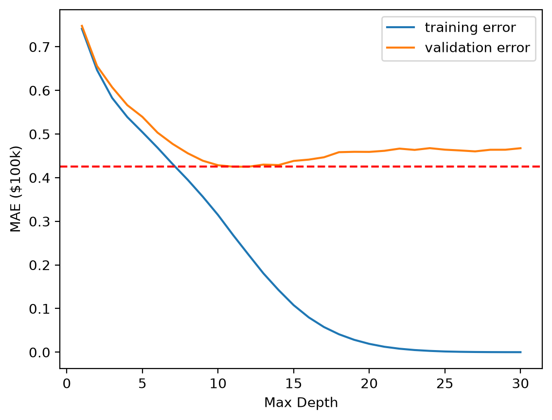
print(f"The lowest validation error: {lowest_validation_error:.3f}")The lowest validation error: 0.425best_depth = depth_list[validation_errors.index(lowest_validation_error)]
print(f"The max_depth value that gives the lowest validation error: {best_depth}")The max_depth value that gives the lowest validation error: 12max_depth=12 gives the lowest validation error, although depths from about 10 to 14 are almost as good. For smaller depths the model underfits, and for larger depths it overfits.
The depth is chosen, so the development is finished. As in section 2, we retrain the tree with this depth on the whole development set and use the test set once, to estimate how well the model predicts new data:
final_model = DecisionTreeRegressor(random_state=0, max_depth=best_depth)
final_model.fit(X_dev, y_dev)

test_error = mean_absolute_error(y_test, final_model.predict(X_test))
print(f"Test error: {test_error:.3f}")
Test error: 0.434YOUR TURN
However, if in the Regression notebook the random forest achieved an error around 0.30–0.35, while our best decision tree still gives about 0.43, does that mean we are still underfitting?
# JUST THINK, NO NEED WRITE, THE SOLUTION IS BELOWNot in the usual sense. Underfitting shows as a high training error, and here the training error is already well below the validation error at the best depth (and zero at depth 30). A large gap between the training and the validation error is a sign of high variance: the tree depends a lot on the particular samples it was trained on.
A single tree cannot have low bias and low variance at the same time. A shallow tree misses patterns in the data, and a deep tree also learns patterns that exist only in its training data. A random forest averages many deep trees, each trained on a different random sample of the data. Their errors partly cancel out, so the variance goes down while each tree stays deep. You will see how this works in Module 5.
Underfitting and overfitting sit at the heart of machine learning. It takes time and practice to fully grasp them, and you will revisit these ideas many times in this course and beyond. Whenever you evaluate a model, take a moment to reflect on how well it fits the data. A solid understanding of these concepts is essential for building and assessing reliable models.
8. Evaluating Classification Models
The first step when working with classification models is to check how many classes you have and how they are distributed. We start with the simplest case, binary classification.
If the dataset has about 50 percent positive and 50 percent negative classes, the classes are balanced. The further this ratio moves away from fifty-fifty, the more imbalance there is. There is no strict rule, but you can think of 70 to 30 as moderate imbalance, 80 to 20 as strong, 90 to 10 as severe, and 99 to 1 as extreme. We will not study class imbalance in detail in this course, but be aware that highly skewed distributions require special attention when building models.
A very important point is to keep the class proportions consistent when splitting the dataset. Until now we have been splitting randomly without checking the distribution. Let us compare the class ratios before and after the train-test split to see what might happen.
X, y = load_breast_cancer(as_frame=True, return_X_y=True)
y = 1 - y # flip the labels: malignant = 1 (positive class), benign = 0
y.value_counts()/y.size
target
0 0.627417
1 0.372583
Name: count, dtype: float64scikit-learn encodes this dataset as malignant = 0 and benign = 1. Above, we flipped the labels with y = 1 - y, so that the positive class (1) is malignant, the class we want to detect. This makes the true and false positives below easier to interpret.
37.3% positive (malignant), 62.7% negative (benign), a moderate imbalance. Now let’s see if we have the same proportions after the split:
X_train, X_test, y_train, y_test = train_test_split(X, y, test_size=0.2, random_state=0)y_train.value_counts()/y_train.sizetarget
0 0.637363
1 0.362637
Name: count, dtype: float64y_test.value_counts()/y_test.sizetarget
0 0.587719
1 0.412281
Name: count, dtype: float64As you can see, the proportions are still close but no longer match the original distribution exactly. To keep the class ratios the same in both the train and test sets, we use a technique called stratification. Scikit learn makes this easy to apply.
X_train, X_test, y_train, y_test = train_test_split(X, y, test_size=0.2, random_state=0, stratify=y) # use the stratify parametery_train.value_counts()/y_train.sizetarget
0 0.626374
1 0.373626
Name: count, dtype: float64y_test.value_counts()/y_test.sizetarget
0 0.631579
1 0.368421
Name: count, dtype: float64As you can see, the proportions are very close to the original X and y, but not exactly the same. Why is that? Take a moment to reflect.
You should apply this idea to all types of splits, including cross-validation, especially when the class imbalance is large.
Now it is time to move beyond accuracy and look at the confusion matrix. First, we will repeat the usual steps: train the model, make predictions, and calculate the accuracy.
# train
model = RandomForestClassifier(random_state=0)
model.fit(X_train, y_train)

# test
y_pred = model.predict(X_test)
accuracy_score(y_test, y_pred)0.9473684210526315Accuracy tells us how often a model makes correct predictions. However, a correct prediction can happen in two different ways:
- The patient actually has cancer and the model predicts cancer (True Positive)
- The patient does not have cancer and the model predicts no cancer (True Negative)
Likewise, there are two different ways the model can be wrong:
- The model predicts cancer even though the patient is healthy (False Positive)
- The model predicts no cancer even though the patient is sick (False Negative)
To see why this distinction matters, imagine two models that both achieve 95 percent accuracy.
In the first model, all of the 5 percent errors are False Positives. In the second model, all of the 5 percent errors are False Negatives.
Even though the accuracy is identical, the consequences of the mistakes are completely different. A model that often gives False Positives leads to unnecessary stress and extra tests. A model that gives False Negatives can miss real cases of cancer. This is why accuracy alone is not enough to evaluate a model.
We can obtain TP, TN, FP and FN in a confusion matrix:
from sklearn.metrics import confusion_matrix
cm = confusion_matrix(y_test, y_pred, labels=model.classes_)

# this will return
# array([[TN,  FP],
#        [FN,  TP]])
cm
array([[67, 5],
[ 1, 41]])print("Correct predictions")
print(f"TN: {cm[0, 0]}")
print(f"TP: {cm[1, 1]}")
print("Wrong predictions")
print(f"FP: {cm[0, 1]}")
print(f"FN: {cm[1, 0]}")Correct predictions
TN: 67
TP: 41
Wrong predictions
FP: 5
FN: 1we can view this better with ConfusionMatrixDisplay
from sklearn.metrics import ConfusionMatrixDisplay
disp = ConfusionMatrixDisplay(cm, display_labels=model.classes_)
disp.plot()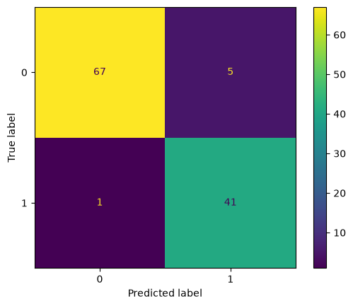
Now we might want to understand how many of the positive predictions were actually correct, or how many of the actual positive cases the model managed to detect. These are called precision and recall.
precision = cm[1, 1]/np.sum(y_pred)
recall = cm[1, 1]/np.sum(y_test)
print(f"Precision: {precision:.3f}") # TP/Positive Predictions
print(f"Recall: {recall:.3f}") # TP/Positive Labels
Precision: 0.891
Recall: 0.976We are not going to define all these metrics one by one as there are many and you can read them here as you need:
https://en.wikipedia.org/wiki/Evaluation_of_binary_classifiers
The most important one you need to understand is the F1 score, which is the harmonic mean of the precision and recall.
\[ F_1 = 2 \cdot \frac{\text{Precision} \cdot \text{Recall}}{\text{Precision} + \text{Recall}} \]
f1 = 2 * (precision * recall) / (precision + recall)
print(f"F1 score: {f1:.4f}")
F1 score: 0.9318In many cases, optimizing the F1 score is a better strategy than optimizing accuracy. Accuracy can appear high simply because of class imbalance, but the F1 score is much harder to fool this way, because it depends on both the precision and the recall of the class it is computed for. It still ignores the correctly predicted negatives, so look at the confusion matrix as well.
And yes, it is implemented in scikit learn so you don’t have to calculate like I did:
from sklearn.metrics import f1_score
f1 = f1_score(y_test, y_pred)
print(f"F1 score: {f1:.4f}")
F1 score: 0.9318you can also use classification_report to get all these at once.
from sklearn.metrics import classification_report
print(classification_report(y_test, y_pred))
precision recall f1-score support
0 0.99 0.93 0.96 72
1 0.89 0.98 0.93 42
accuracy 0.95 114
macro avg 0.94 0.95 0.94 114
weighted avg 0.95 0.95 0.95 114
You can see in the classification report that the f1-score is shown separately for class 0 and class 1. The value we calculated earlier corresponds only to the positive class. Why is that?
Since the f1-score is an important metric, it is useful to understand it in more depth. Please read the following:
- https://en.wikipedia.org/wiki/F-score
- https://scikit-learn.org/stable/modules/generated/sklearn.metrics.f1_score.html
Pay special attention to the pos_label and average parameters in the scikit-learn documentation, as these determine which class is treated as positive and how the overall score is aggregated.
Answer
By default, f1_score treats the problem as binary and computes the F1 score of one class only, the positive class pos_label=1. Precision and recall are defined for one class: for the positive class, precision asks how many of the predicted positives are correct. The classification report computes the same score for each class in turn, treating it as the positive class, and then averages them in the macro avg and weighted avg rows.
More than two classes. With more than two classes, such as the four vehicle types in the Classification notebook, there is one F1 score per class. The average parameter of f1_score decides how they become one number:
average="macro": the plain mean of the per-class F1 scores. Every class counts equally, however rare it is.average="weighted": the mean weighted by the number of samples in each class, so frequent classes dominate.average="micro": computed from the counts over all classes; for problems with one label per sample it equals accuracy.
Macro-F1 punishes a model that neglects a small class, which accuracy and weighted F1 can hide. A model that always predicts the majority class can reach a decent accuracy, but its macro-F1 is low, because the F1 of every other class is 0. The macro avg and weighted avg rows of the classification report above are exactly these averages.
Class probabilities
A final important evaluation approach for classification models is to look at their predicted probabilities. So far, we have only seen models output 0s and 1s, but most classifiers can also provide the probability of each class. This is helpful because it tells us how confident the model is in its prediction.
Think of it like this: probabilities above 50 percent are typically interpreted as the positive class, and below 50 percent as the negative class. But a prediction made with 99 percent confidence is very different from one made with 60 percent confidence, even though both would still be classified as positive.
You can use the .predict_proba() method instead of .predict() to obtain the predicted probabilities for each class.
# col 0: probability of class 0
# col 1: probability of class 1
model.predict_proba(X_test)
array([[0.95, 0.05],
[0.86, 0.14],
[0.91, 0.09],
[0.98, 0.02],
[0.92, 0.08],
[0.01, 0.99],
[1. , 0. ],
[0.71, 0.29],
[0.33, 0.67],
[0.97, 0.03],
[0.96, 0.04],
[0. , 1. ],
[0. , 1. ],
[0.99, 0.01],
[0. , 1. ],
[1. , 0. ],
[1. , 0. ],
[0.85, 0.15],
[1. , 0. ],
[0.28, 0.72],
[0.05, 0.95],
[0.06, 0.94],
[0.01, 0.99],
[0. , 1. ],
[0. , 1. ],
[0.94, 0.06],
[1. , 0. ],
[1. , 0. ],
[1. , 0. ],
[0.01, 0.99],
[0.99, 0.01],
[0. , 1. ],
[0.6 , 0.4 ],
[0. , 1. ],
[1. , 0. ],
[1. , 0. ],
[0.99, 0.01],
[1. , 0. ],
[1. , 0. ],
[0. , 1. ],
[0.38, 0.62],
[0.99, 0.01],
[1. , 0. ],
[0.02, 0.98],
[0.62, 0.38],
[0.97, 0.03],
[1. , 0. ],
[0.96, 0.04],
[0.21, 0.79],
[0.9 , 0.1 ],
[1. , 0. ],
[1. , 0. ],
[1. , 0. ],
[1. , 0. ],
[1. , 0. ],
[0.01, 0.99],
[0.11, 0.89],
[0.41, 0.59],
[1. , 0. ],
[0.94, 0.06],
[0.99, 0.01],
[0.02, 0.98],
[0.89, 0.11],
[0. , 1. ],
[0.29, 0.71],
[0.99, 0.01],
[1. , 0. ],
[0. , 1. ],
[0. , 1. ],
[0.82, 0.18],
[0.37, 0.63],
[1. , 0. ],
[0.9 , 0.1 ],
[0.97, 0.03],
[0.85, 0.15],
[0. , 1. ],
[0.06, 0.94],
[0.12, 0.88],
[1. , 0. ],
[0.83, 0.17],
[1. , 0. ],
[1. , 0. ],
[1. , 0. ],
[1. , 0. ],
[0.02, 0.98],
[0. , 1. ],
[0.01, 0.99],
[0.88, 0.12],
[1. , 0. ],
[0.03, 0.97],
[1. , 0. ],
[0.01, 0.99],
[0. , 1. ],
[1. , 0. ],
[0.93, 0.07],
[1. , 0. ],
[0. , 1. ],
[0.01, 0.99],
[0.38, 0.62],
[0.84, 0.16],
[0. , 1. ],
[0.83, 0.17],
[0.01, 0.99],
[0.01, 0.99],
[1. , 0. ],
[1. , 0. ],
[0.02, 0.98],
[0.06, 0.94],
[0.31, 0.69],
[1. , 0. ],
[0.91, 0.09],
[0.98, 0.02],
[0.02, 0.98],
[1. , 0. ]])How can we evaluate whether these so-called probabilities are truly probabilities?
For example, imagine the weather forecast says there is a 90 percent chance of rain tomorrow, but then it doesn’t rain. Does this mean the forecast was wrong? Not necessarily. A 90 percent probability means that on average, out of 10 days with a “90 percent rain” forecast, it should rain on about 9 of them. So a single day not raining tells us nothing.
To evaluate whether the probability is good, we must look at all the days where the forecast predicted 90 percent rain and check what fraction of those days actually had rain. If the proportion is close to 0.9, the forecast is well-calibrated.
We can apply the exact same idea to our machine learning models. This is called calibration. A model is well-calibrated when, among all predictions where the model outputs a probability of 0.7, roughly 70 percent of them are actually positive.
Calibration is extremely important in real applications, but it is also quite advanced for this course. We will not study it in detail here, but curious students can explore more in the documentation:
https://scikit-learn.org/stable/modules/calibration.html
9. Evaluating Regression Models
When working with regression models, we again start by understanding the target variable we want to predict. Just like class imbalance matters in classification, the distribution of the target affects how we evaluate regression models.
If the target is skewed, has extreme outliers, or spans a very large numerical range, certain metrics become more sensitive than others. Before training any model, always inspect the target distribution.
X, y = load_diabetes(as_frame=True, return_X_y=True)
plt.hist(y)
(array([38., 80., 68., 62., 50., 41., 38., 42., 17., 6.]),
array([ 25. , 57.1, 89.2, 121.3, 153.4, 185.5, 217.6, 249.7, 281.8,
313.9, 346. ]),
<BarContainer object of 10 artists>)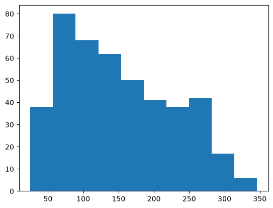
In classification, we use stratification to preserve class proportions. Regression has no discrete classes, but we still want the train and test sets to contain similar ranges of target values. If the target contains extreme or rare values, a purely random split might place all high values in the training set or all low values in the test set.
In the load_diabetes dataset, the target distribution is not very skewed, so even a simple random split gives y_train and y_test that look fairly similar. However, it is still useful to know how to control this. A common approach is to bin the continuous target variable and then stratify based on those bins.
# bin the target into quantiles
y_bins = pd.qcut(y, q=10)
y_bins
0 (140.5, 168.0]
1 (60.0, 77.0]
2 (140.5, 168.0]
3 (196.7, 232.0]
4 (115.0, 140.5]
...
437 (168.0, 196.7]
438 (94.0, 115.0]
439 (115.0, 140.5]
440 (196.7, 232.0]
441 (24.999, 60.0]
Name: target, Length: 442, dtype: category
Categories (10, interval[float64, right]): [(24.999, 60.0] < (60.0, 77.0] < (77.0, 94.0] < (94.0, 115.0] ... (168.0, 196.7] < (196.7, 232.0] < (232.0, 265.0] < (265.0, 346.0]]# stratified split based on bins
X_train, X_test, y_train, y_test = train_test_split(X, y, test_size=0.2, random_state=0, stratify=y_bins)# target distribution in y, y_train, y_test
plt.hist(y, label='y', histtype='step')
plt.hist(y_train, label='y_train', histtype='step')
plt.hist(y_test, label='y_test', histtype='step')
plt.legend()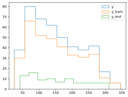
Now we can build our model and evaluate it beyond MAE. Regression has no confusion matrix, but there are several common metrics that each reveal a different aspect of the model’s performance.
from sklearn.ensemble import RandomForestRegressor
model = RandomForestRegressor(random_state=0)
model.fit(X_train, y_train)RandomForestRegressor(random_state=0)In a Jupyter environment, please rerun this cell to show the HTML representation or trust the notebook.
On GitHub, the HTML representation is unable to render, please try loading this page with nbviewer.org.
Parameters
Fitted attributes
from sklearn.metrics import mean_absolute_error, mean_squared_error
y_pred = model.predict(X_test)
mae = mean_absolute_error(y_test, y_pred)
mse = mean_squared_error(y_test, y_pred)
rmse = np.sqrt(mse)

print(f"Mean Absolute Error: {mae:.4f}")
print(f"Mean Squared Error: {mse:.4f}")
print(f"Root Mean Squared Error: {rmse:.4f}")
Mean Absolute Error: 47.9390
Mean Squared Error: 3569.1825
Root Mean Squared Error: 59.7426- Mean Absolute Error (MAE): The average absolute difference between predicted and actual values.
- Mean Squared Error (MSE): The average squared difference. Large errors are punished very strongly.
- Root Mean Squared Error (RMSE): The square root of MSE. Same unit as the target.
To understand the difference between MAE and RMSE, let’s look at a dummy example
ground_truth = np.array([10, 10, 10, 10])
case_1 = np.array([12, 16, 12, 16]) # errors are 2, 6, 2, 6
case_2 = np.array([14, 14, 14, 14]) # errors are 4, 4, 4, 4
# MAE
print("--MAE--")
print("case 1 mae: ", mean_absolute_error(ground_truth, case_1))
print("case 2 mae: ", mean_absolute_error(ground_truth, case_2))--MAE--
case 1 mae: 4.0
case 2 mae: 4.0MAE treats both predictions as equally good, even though one model makes larger individual errors. RMSE, on the other hand, penalizes large errors more strongly, so it can distinguish between these cases even when the MAE is the same.
# RMSE
print("--RMSE--")
print("case 1 rmse: ", np.sqrt(mean_squared_error(ground_truth, case_1)))
print("case 2 rmse: ", np.sqrt(mean_squared_error(ground_truth, case_2)))
--RMSE--
case 1 rmse: 4.47213595499958
case 2 rmse: 4.0There is no universal “better” metric, it depends on the problem. They measure error in different ways:
- MAE treats all errors equally. It is easier to interpret and more robust to outliers.
- RMSE penalizes large errors more. It is useful when large mistakes are especially costly and you want the model to avoid them.
So the choice depends on what you care about:
- If avoiding big errors is important, RMSE is more appropriate.
- If you want a stable, easy-to-interpret measure that is less sensitive to outliers, MAE is more appropriate.
As you have seen in the Regression notebook, plotting the predictions vs labels is useful:
plt.scatter(y_test, y_pred)
plt.xlim(0, 350)
plt.ylim(0, 350)
plt.plot([0, 350], [0, 350], label='perfect prediction line', linestyle='--')
plt.xlabel("Labels (y_test)")
plt.ylabel("Predictions (y_pred)")
plt.legend()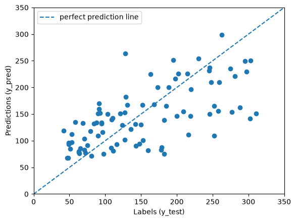
we can extend this analysis by plotting the residuals, i.e. the differences between the true and predicted values.
plt.scatter(y_test, y_pred, s=15)

# Add x = y diagonal
min_val = min(y_test.min(), y_pred.min())
max_val = max(y_test.max(), y_pred.max())
plt.plot([min_val, max_val], [min_val, max_val], linestyle='--', linewidth=0.7, color='black')

# Draw residual lines
for yt, yp in zip(y_test, y_pred):
    plt.plot([yt, yt], [yt, yp], color='gray', linewidth=0.3)

plt.xlabel("y_test")
plt.ylabel("y_pred")
plt.title("Predicted vs True with Residuals")
plt.show()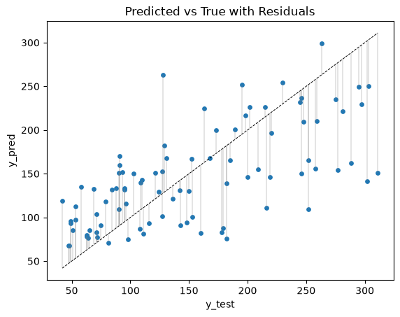
residuals = y_test - y_pred

plt.scatter(y_pred, residuals)
plt.axhline(0, color="black")
plt.xlabel("Predicted")
plt.ylabel("Residual")
plt.ylim(-200, 200)
plt.title("Residuals vs Predicted Values")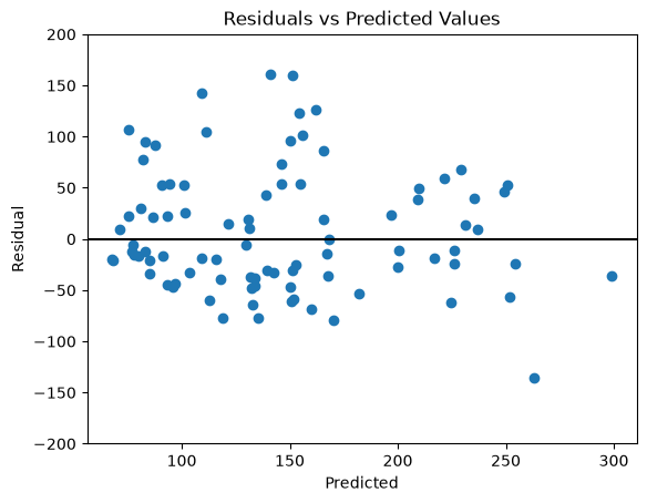
For a well-behaving model, residuals should appear random. If you notice patterns such as consistently positive or consistently negative errors, or errors that grow with the target value, this indicates the model is biased or missing important structure, and further investigation is needed.
Finally, regression models do not output probabilities like classification models do. Instead, we talk about uncertainty. Rather than giving a single point estimate such as 30k, a regression model can also express how confident it is by providing a range, for example 30k ± 5k. This interval reflects how uncertain the model is about the prediction.
A simple way to illustrate this idea is to train many models, each with a different random_state. For a single test data point, you collect predictions from all the trained models, compute their mean, and report the middle 95% of these predictions as a range. This shows how much the predictions vary with the model’s randomness. Note that this is not a real prediction interval, which would also have to account for the noise in the data itself, but it gives a first feeling for how uncertain the model is.
# train 50 models on the same training data
models = []
for i in range(50):
    m = RandomForestRegressor(random_state=i)
    m.fit(X_train, y_train)
    models.append(m)
# get 50 predictions on a single data point
datapoint_index = 0
preds = np.array([m.predict(X_test.iloc[datapoint_index:datapoint_index+1])[0] for m in models])lower = np.percentile(preds, 2.5)
upper = np.percentile(preds, 97.5)
point = np.mean(preds)
print("Label: ", y_test.iloc[datapoint_index:datapoint_index+1].tolist()[0])
print(f"Prediction: {point:.2f} ({lower:.2f}-{upper:.2f})")Label: 178.0
Prediction: 82.83 (75.50-91.91)The label, 178, lies far outside this range. The range only shows how much the forest’s predictions vary with its random seed. It says nothing about how far a prediction can be from the truth; a real prediction interval also has to account for that.
Uncertainty quantification is a large topic in both classification and regression. It is a topic of its own. For now, remember the key idea: we usually make point estimates, but these estimates are much more meaningful when combined with an uncertainty interval. A prediction of 80% ± 0.1% means something very different from 80% ± 5%.
For students who want to explore further, here are some useful starting points:
10. Exercises
YOUR TURN
- California Housing (Regression)
- Load the California housing dataset.
- Split the data into dev and test sets.
- On the dev set, build the best model you can using:
- feature selection and feature engineering
- model selection
- hyperparameter tuning with Optuna
- cross validation for evaluation
- Once you identify the best model, fit it on the full dev set, then evaluate thoroughly on the test set (metrics, plots, error analysis).
- Vehicle (Classification)
- Repeat the same for classification, with the vehicle dataset of the Classification notebook:
fetch_openml(name="vehicle", version=1, as_frame=True, return_X_y=True), and macro-F1 as the metric.
California Housing has about 20,000 rows, so a random forest tuned with Optuna and 5-fold cross-validation can take a long time. Start with a few trials or a sample of the rows, or use HistGradientBoostingRegressor, which is much faster.
To give you an idea of what is possible, without telling you what to reach: on the development set, HistGradientBoostingRegressor with default settings has a cross-validated MAE of about 0.32 on California Housing, and a default random forest reaches a cross-validated macro-F1 of about 0.74 on the vehicle data. Feature engineering and tuning can improve on both.
# YOUR CODE HERE