from pathlib import Path
import numpy as np
import pandas as pd
import matplotlib.pyplot as plt
import matplotlib

print("pandas version:", pd.__version__)
print("numpy version:", np.__version__)
print("matplotlib version:", matplotlib.__version__)Regression

In the Classification notebook, you went through the whole CRISP-DM cycle once, with a classification model. In this notebook you go through it again with a regression model, on the same dataset. The steps that are the same as in Classification are short here, so you can focus on what changes: the targets, the baseline and the metric.
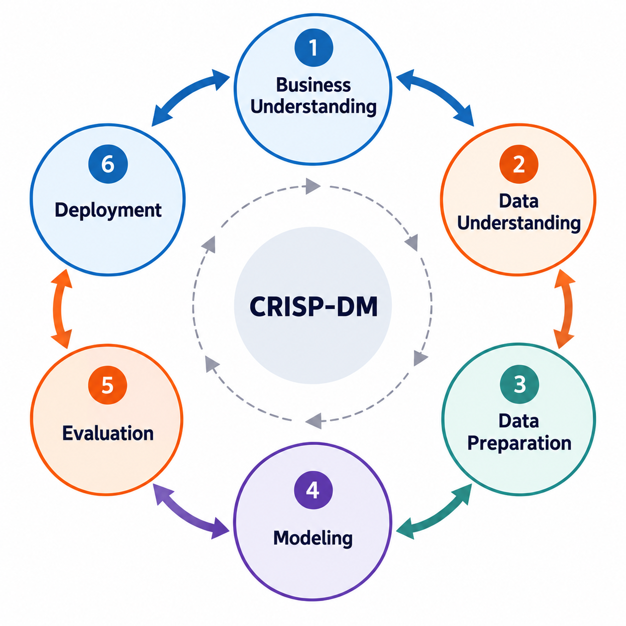
- Phase 1 – Business Understanding: ✅ Done.
- Phase 2 – Data Understanding: ✅ Done, in the Classification notebook.
- Phase 3 – Data Preparation: As in Classification, with other targets.
- Phase 4 – Modelling: Train regression models to predict the energy levels
homoandlumo. - Phase 5 – Evaluation: Assess the performance of your trained models.
- Phase 6 – Deployment: Save the trained models for future use.
1. Business Understanding
Done ✅ You read the Business Understanding page.
2. Data Understanding
Done ✅ You read the Data Understanding page and explored the dataset in the Classification notebook.
Your Turn
Read starter_dataset.xlsx into the df variable, as in the Classification notebook.
Working in Colab? The repository’s
data/folder is not available there. Pandas can read the file directly from GitHub instead:pd.read_excel("https://raw.githubusercontent.com/BredaUniversityADSAI/introduction-to-ml/stable/data/002_processed_data/starter_dataset.xlsx")
# YOUR CODE HEREYour exploration in the Classification notebook did not depend on the task, so it holds here as well. Look back at what you found about homo and lumo: their distributions, their missing values, and how they relate to each other.
3. Data Preparation
The dataset is already prepared, so this section is short. The difference with Classification is the target: you use the same features, but predict homo and lumo instead of stability.
Your Turn
You first predict lumo, and later in this notebook homo. A row without a value for the target you predict is of no use, but a row with only homo (or stability) missing still has a good lumo label.
Keep a copy of the full data (for example df_all = df.copy()), then remove the rows where lumo is missing (NaN). How many molecules are left? For the HOMO model in section 6, you start again from df_all and remove the rows where homo is missing.
# YOUR CODE HEREYour Turn
Prepare the columns as in Classification, with one difference:
- Keep
homo,lumoandstabilityout of the input features: they are the targets. A target is not known for a new molecule, so a model that uses one as a feature would look good in testing and could not be used (data leakage). - Drop the column
smiles, since it is not an input to the model.
# YOUR CODE HERE4. Modelling
df.head()We have two target variables: homo and lumo. There are two possible approaches: either train a single model to predict both simultaneously or train separate models for each target. In this section, we will focus on building a model to predict lumo. At the end, in section 6, you will be asked to build a similar model for predicting homo.
Your Turn
Create the input features X (the molecular descriptor columns) and set the target variable y to the lumo column.
# YOUR CODE HEREIn Classification, the baseline always predicted the majority class. For regression, a common baseline is to always predict the mean of the target variable, and its performance is measured with an error metric such as the Mean Absolute Error (MAE).
Your Turn
Calculate the MAE you would achieve if you always predict the mean of y. As in Classification, you can use all of y for this first quick estimate; strictly speaking, compute the mean on the training set only (y_train.mean()) and measure its MAE on the test set.
# YOUR CODE HEREYour Turn
Split the data into training and test sets as in Classification (80 percent training, 20 percent test, random_state=42) and check the shapes.
# YOUR CODE HEREYour Turn
Import the RandomForestRegressor from sklearn.ensemble, the regression version of the RandomForestClassifier you used in Classification. Create it with random_state=42 and fit it on the training data.
# YOUR CODE HERE5. Evaluation
As in Classification, you evaluate the model on the test set, which it has not seen during training.
Your Turn
Predict the test set and save the predictions in y_pred.
# YOUR CODE HEREYour Turn
Evaluate the model’s performance using scikit-learn’s built-in metrics. Import mean_absolute_error from sklearn.metrics, calculate the mean absolute error by comparing y_test and y_pred, and report the result in 3 decimal places.
# YOUR CODE HEREIs the model better than the baseline?
Your Turn
As in Classification, create a DataFrame that compares the predictions (y_pred) with the true values (y_test). For which molecules is the error largest?
# YOUR CODE HERE6. Modelling and Evaluation (HOMO predictor)
Start again from the full data and remove the rows where homo is missing. Build a second model to predict homo and evaluate its performance using the mean absolute error on the test set. Create a baseline by calculating the Mean Absolute Error (MAE) when predicting the mean of y for all observations. Then compare each model with its own baseline. The MAEs of the two models are not directly comparable, because homo and lumo have different spreads: which model improves more on its baseline?
# YOUR CODE HERE7. Deployment
Save your models in the models folder, as in Classification. Remember the extra step from the Classification notebook: once you are done with testing, retrain each model on all of its data before you save it.
Your Turn
This time you have two models. Retrain the models on the entire dataset and save them as
homo_iteration1.jobliblumo_iteration1.joblib
under the folder models.
# YOUR CODE HERE