import numpy as np
import pandas as pd
import matplotlib.pyplot as pltData Preparation

Data preparation is the process of cleaning, transforming, and organizing raw data into a suitable format for machine learning models, ensuring that the algorithms can learn effectively and produce reliable results.
In CRISP-DM, Data Preparation comes after Data Understanding, but in this course you learn it first. Exploring a dataset often needs prepared data, for example scaled or encoded features, so the next notebook, Data Understanding, uses the tools from this one. The End-to-End ML Project notebook explains this order in more detail.
Outline:
- Motivation
- Feature Scaling
- Feature Transformations
- Missing Data
- Merging Data
- Encoding Data
- Exercise
1. Motivation
Before diving into the details, I want you to avoid a common misconception: that improving machine learning pipeline performance is mainly about choosing or tuning models. In reality, proper data preparation, even with the exact same model, can be the key difference between weak and strong results. Every phase of the CRISP-DM cycle is important.
Let’s load our housing data and see an example:
from sklearn.datasets import fetch_california_housing
X, y = fetch_california_housing(as_frame=True, return_X_y=True)
I’ll load a model we haven’t studied yet, a Support Vector Machine. By now, you’ve seen that loading different models in scikit-learn follows the same simple pattern. You don’t need to understand how this particular algorithm works; just think of it as another machine learning model for demonstration purposes.
from sklearn.svm import SVR
model = SVR()
and train/test it on the dataset:
from sklearn.model_selection import train_test_split
from sklearn.metrics import mean_absolute_error

# split
X_train, X_test, y_train, y_test = train_test_split(X, y, test_size=0.2, random_state=0)
# fit
model.fit(X_train, y_train)
# test
y_pred = model.predict(X_test)
mae = mean_absolute_error(y_test, y_pred)
print(mae)0.8609461073379858That’s quite a large error compared to our initial results.
Now let’s scale the data. We’ll discuss what scaling means in a moment, for now, just understand that we’re applying a data preparation step to improve the model’s performance.
# scale the data
from sklearn.preprocessing import StandardScaler
scaler = StandardScaler()
X_train = scaler.fit_transform(X_train)
X_test = scaler.transform(X_test)
# repeat
# call the model again
model = SVR()
# fit
model.fit(X_train, y_train)
# test
y_pred = model.predict(X_test)
mae = mean_absolute_error(y_test, y_pred)
print(mae)0.38556904660770236The error dropped from $86K to $39K, almost a $50K reduction in house price prediction error, just by applying one data preparation step. This shows how critical proper data preparation is, as models can perform poorly without producing any error messages to indicate what went wrong.
2. Feature Scaling
What we applied above is a feature scaling technique called standardization. Feature scaling is one of the most common data preparation steps in both machine learning and deep learning. Rather than defining it right away, let’s first observe its effect and discuss what it means afterward.
scaler = StandardScaler()
X_scaled = scaler.fit_transform(X)
Note that scikit-learn transformers return a NumPy array by default, even when the input was a pandas DataFrame, so the column names are lost. Most transformers can return a DataFrame instead if you ask for it, for example StandardScaler().set_output(transform="pandas"), but in this course we mostly work with the default.
type(X), type(X_scaled)(pandas.DataFrame, numpy.ndarray)X.head()| MedInc | HouseAge | AveRooms | AveBedrms | Population | AveOccup | Latitude | Longitude | |
|---|---|---|---|---|---|---|---|---|
| 0 | 8.3252 | 41.0 | 6.984127 | 1.023810 | 322.0 | 2.555556 | 37.88 | -122.23 |
| 1 | 8.3014 | 21.0 | 6.238137 | 0.971880 | 2401.0 | 2.109842 | 37.86 | -122.22 |
| 2 | 7.2574 | 52.0 | 8.288136 | 1.073446 | 496.0 | 2.802260 | 37.85 | -122.24 |
| 3 | 5.6431 | 52.0 | 5.817352 | 1.073059 | 558.0 | 2.547945 | 37.85 | -122.25 |
| 4 | 3.8462 | 52.0 | 6.281853 | 1.081081 | 565.0 | 2.181467 | 37.85 | -122.25 |
# similar to .head()
X_scaled[:5, :]
array([[ 2.34476576, 0.98214266, 0.62855945, -0.15375759, -0.9744286 ,
-0.04959654, 1.05254828, -1.32783522],
[ 2.33223796, -0.60701891, 0.32704136, -0.26333577, 0.86143887,
-0.09251223, 1.04318455, -1.32284391],
[ 1.7826994 , 1.85618152, 1.15562047, -0.04901636, -0.82077735,
-0.02584253, 1.03850269, -1.33282653],
[ 0.93296751, 1.85618152, 0.15696608, -0.04983292, -0.76602806,
-0.0503293 , 1.03850269, -1.33781784],
[-0.012881 , 1.85618152, 0.3447108 , -0.03290586, -0.75984669,
-0.08561576, 1.03850269, -1.33781784]])As a result, the transformed data no longer retains the original column names or index, though the column order remains the same. If we want to keep the familiar structure, we can easily recreate a DataFrame using the original column names.
X_scaled = pd.DataFrame(X_scaled, columns=X.columns)
X_scaled.head()| MedInc | HouseAge | AveRooms | AveBedrms | Population | AveOccup | Latitude | Longitude | |
|---|---|---|---|---|---|---|---|---|
| 0 | 2.344766 | 0.982143 | 0.628559 | -0.153758 | -0.974429 | -0.049597 | 1.052548 | -1.327835 |
| 1 | 2.332238 | -0.607019 | 0.327041 | -0.263336 | 0.861439 | -0.092512 | 1.043185 | -1.322844 |
| 2 | 1.782699 | 1.856182 | 1.155620 | -0.049016 | -0.820777 | -0.025843 | 1.038503 | -1.332827 |
| 3 | 0.932968 | 1.856182 | 0.156966 | -0.049833 | -0.766028 | -0.050329 | 1.038503 | -1.337818 |
| 4 | -0.012881 | 1.856182 | 0.344711 | -0.032906 | -0.759847 | -0.085616 | 1.038503 | -1.337818 |
Now let’s examine one of the columns, HouseAge, to see how it changes before and after scaling.
fig, ax = plt.subplots(1, 2, figsize=(10, 5))
ax[0].hist(X['HouseAge'])
ax[0].set_xlabel('HouseAge')
ax[1].hist(X_scaled['HouseAge'])
ax[1].set_xlabel('HouseAge (Scaled)')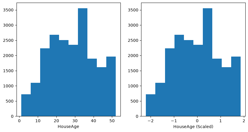
Everything looks the same except for the values on the x-axis: the overall shape of the distribution is identical, but after scaling it is centered around zero with a standard deviation close to one.
This is the case for all the columns:
X_scaled.mean()MedInc 5.508083e-17
HouseAge 4.406467e-17
AveRooms 7.711317e-17
AveBedrms -1.005225e-16
Population -1.101617e-17
AveOccup 0.000000e+00
Latitude 2.247298e-15
Longitude -8.603626e-15
dtype: float64X_scaled.std()MedInc 1.000024
HouseAge 1.000024
AveRooms 1.000024
AveBedrms 1.000024
Population 1.000024
AveOccup 1.000024
Latitude 1.000024
Longitude 1.000024
dtype: float64another type of feature scaling is min-max scaling also called normalization.
from sklearn.preprocessing import MinMaxScaler
scaler = MinMaxScaler()
X_scaled = scaler.fit_transform(X)
X_scaled = pd.DataFrame(X_scaled, columns=X.columns)fig, ax = plt.subplots(1, 2, figsize=(10, 5))
ax[0].hist(X['HouseAge'])
ax[0].set_xlabel('HouseAge')
ax[1].hist(X_scaled['HouseAge'])
ax[1].set_xlabel('HouseAge (Scaled)')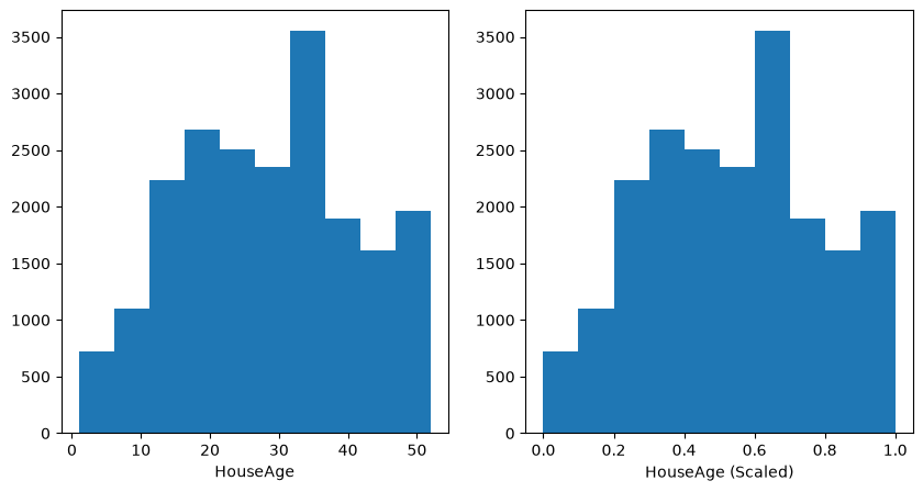
What is the difference? The feature values have been rescaled to lie between 0 (the minimum) and 1 (the maximum), which is why this method is called min-max scaling. You can adjust the scaler’s parameters to set a different minimum and maximum range if needed.
scaler = MinMaxScaler(feature_range=(-1, 1)) # let's change the range
X_scaled = scaler.fit_transform(X)
X_scaled = pd.DataFrame(X_scaled, columns=X.columns)
fig, ax = plt.subplots(1, 2, figsize=(10, 5))
ax[0].hist(X['HouseAge'])
ax[0].set_xlabel('HouseAge')
ax[1].hist(X_scaled['HouseAge'])
ax[1].set_xlabel('HouseAge (Scaled)')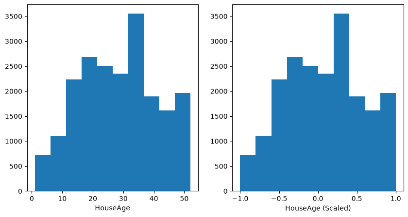
X_scaled.min()MedInc -1.0
HouseAge -1.0
AveRooms -1.0
AveBedrms -1.0
Population -1.0
AveOccup -1.0
Latitude -1.0
Longitude -1.0
dtype: float64X_scaled.max()MedInc 1.0
HouseAge 1.0
AveRooms 1.0
AveBedrms 1.0
Population 1.0
AveOccup 1.0
Latitude 1.0
Longitude 1.0
dtype: float64Now we can define what feature scaling is.
Many machine learning algorithms perform poorly when numerical features have very different scales: models based on distances, such as k-nearest neighbors and support vector machines, and models trained with gradient descent. Tree-based models are the main exception. In the Classification notebook, we mentioned that some models require normalization of the input data, while models such as RandomForest and DecisionTree do not. This is precisely why we started with Random Forest, it works well even without scaling. This is also why I selected SVM in the motivation section, because it is sensitive to the scale of the feature values.
There are two common techniques to bring all features to a similar scale: standardization and min-max scaling. Standardization rescales the data so that each feature has a mean of zero and a standard deviation of one. Min-max scaling (sometimes also called normalization; scikit-learn’s Normalizer does something else: it rescales each row, not each column) rescales the data to a fixed range, typically between 0 and 1.
fit_transform vs transform
Before we conclude this section, there is one important detail to understand. Earlier, in the motivation section, we standardized the data using the following code:
from sklearn.preprocessing import StandardScaler
scaler = StandardScaler()
X_train = scaler.fit_transform(X_train)
X_test = scaler.transform(X_test)
YOUR TURN
What is the difference between fit_transform and transform, and why do we apply the first to X_train and the second to X_test?
The answer will be given below but first try to find the answer yourself.
# YOUR ANSWER HERE
# If you prefer write it in markdown.
SOLUTION
When you call fit_transform, the scaler calculates the mean and standard deviation of each feature (this is the “fit” step) and then uses those values to scale the data (the “transform” step). We do this only on the training data, because the model should learn scaling parameters only from the data it has “seen” during training.
When you call transform on the test data, the scaler applies the same mean and standard deviation from the training data, without recalculating them. This ensures that both training and test data are scaled consistently.
If you scaled the entire dataset before splitting, information from the test set would leak into the training process because the mean and standard deviation would include the test data. This is called data leakage, and it can make your model’s performance appear better than it actually is.
Scaling before splitting is a common form of data leakage, and reviewers of a project or a thesis look for it. So always split first, then scale, and remember, this applies to any transformation where parameters are learned from the data.
3. Feature Transformations
Feature scaling is just one type of feature transformation. Some features require transformations that go beyond simple scaling. Let’s see why:
plt.hist(X['Population'])
plt.ylabel('Count')
plt.xlabel('Population')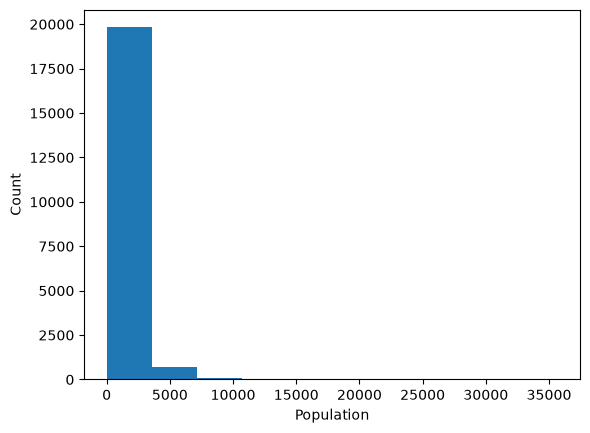
The Population column represents the total number of people living in each California census block group. The distribution is right-skewed, meaning most block groups have populations below 5,000, but a few densely populated areas reach much higher values, up to around 35,000.
We can visually see this from the histogram, but we can quantify with some useful numpy and pandas functionality as well.
np.percentilereturns the value below which a given percentage of data falls, for example, the 99th percentile is the value below which 99% of the data lie. 🔗 NumPy documentationnlargest(in pandas) returns the top n largest values or rows from a Series or DataFrame column. 🔗 pandas documentation
# 99% of block groups have a population below roughly 5,800
np.percentile(X['Population'], 99)np.float64(5805.830000000002)# However, some block groups are much more densely populated
X['Population'].nlargest(5)15360 35682.0
9880 28566.0
13139 16305.0
10309 16122.0
6057 15507.0
Name: Population, dtype: float64Skewed features cause problems for several kinds of models, because a few extreme values have a large influence:
- Models that use distances between samples, such as k-nearest neighbors or k-means, compare samples feature by feature. After standard scaling, the few block groups with a very large population are many standard deviations away from the rest, while most block groups are squeezed together in a narrow range.
- In a linear model, samples with extreme feature values have a large influence on the fitted coefficients, so a handful of block groups can pull the fitted line towards them.
- Many skewed quantities, such as population, income or prices, behave multiplicatively: a change from 100 to 200 people says more about a block group than a change from 10,000 to 10,100. On a logarithmic scale, equal ratios become equal steps, and the relationship with the target is often closer to linear.
A common fix is to apply a logarithmic transformation (log) to the feature. It pulls the large values in and spreads out the small ones.
log_feature = np.log(X['Population'])
plt.hist(log_feature)
(array([3.0000e+00, 2.1000e+01, 8.5000e+01, 1.8700e+02, 6.5600e+02,
4.9080e+03, 1.1631e+04, 2.9050e+03, 2.3800e+02, 6.0000e+00]),
array([ 1.09861229, 2.03699122, 2.97537016, 3.91374909, 4.85212803,
5.79050696, 6.7288859 , 7.66726483, 8.60564377, 9.5440227 ,
10.48240164]),
<BarContainer object of 10 artists>)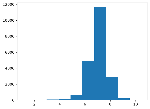
The skew is much reduced: the long tail on the right is gone, and the distribution is close to symmetric, with a small tail on the left.
A log transformation has limits. It does not help a model with values outside the range it was trained on: a population larger than any in the training set is still larger than any in the training set after the log. Tree-based models, which you meet in Module 5, split each feature at a threshold, so a transformation that keeps the order of the values, such as the log, gives the same tree. The log matters most for distance-based and linear models.
YOUR TURN
Can you think of a case where we cannot apply np.log() to skewed data? The answer follows from the definition of the logarithm.
# YOUR ANSWER/CODE HEREHint: the domain of the log function is…?
Answer
The logarithm is only defined for positive numbers: np.log(0) gives -inf and a negative value gives nan. Population is always positive, but a feature with zeros needs np.log1p (the log of 1 + x), and a feature with negative values needs another transformation, such as the signed version in the exercise at the end of this notebook.
YOUR TURN
We discussed that it’s crucial to apply scaling after the train/test split. Do you think the same rule applies to a log transformation? Why or why not?
# YOUR ANSWER
# Use markdown if you want
Answer
No. The rule is about transformations that learn something from the data: a scaler learns the mean and standard deviation, and if it learns them from all the data, the test data influences the training data. A log transformation learns nothing: it is the same function for every value, so it gives the same result before or after the split. Many transformations are fitted, though, so splitting first is the safe habit.
4. Missing Data
Handling missing values with pandas is part of the prerequisites. If you need a reminder, the pandas user guide covers it in depth:
https://pandas.pydata.org/docs/user_guide/missing_data.html
Therefore I will keep this section short, but I would like to emphasize three important points specific to scikit-learn.
Point 1:
Some models can handle missing features natively. For such models, it might be better not to process missing values.
# let's generate dummy data with a single feature that contains one nan value
X = np.array([[-1], [-5], [10], [7], [2], [-7], [np.nan]])
y = np.array([0, 0, 1, 1, 1, 0, 0])
# most models will complain
# please read the error message
model = SVR()
try:
model.fit(X, y)
except Exception as e:
print(e)Input X contains NaN.
SVR does not accept missing values encoded as NaN natively. For supervised learning, you might want to consider sklearn.ensemble.HistGradientBoostingClassifier and Regressor which accept missing values encoded as NaNs natively. Alternatively, it is possible to preprocess the data, for instance by using an imputer transformer in a pipeline or drop samples with missing values. See https://scikit-learn.org/stable/modules/impute.html You can find a list of all estimators that handle NaN values at the following page: https://scikit-learn.org/stable/modules/impute.html#estimators-that-handle-nan-values# but there are a few that could handle nans natively
from sklearn.ensemble import HistGradientBoostingClassifier
clf = HistGradientBoostingClassifier()
clf.fit(X, y)HistGradientBoostingClassifier()In a Jupyter environment, please rerun this cell to show the HTML representation or trust the notebook.
On GitHub, the HTML representation is unable to render, please try loading this page with nbviewer.org.
Parameters
Fitted attributes
Point 2:
If you use models that do not accept missing values (NaNs), you have three main options:
- Drop missing values: Simple and keeps only complete data, but you may lose valuable information if many rows contain
NaNs. - Impute missing values: Replace them with estimated numbers (like the mean or training a model to predict features). This preserves all samples but can introduce bias if the imputation method is not appropriate.
- Fill with a constant (e.g.,
-99): Technically a form of imputation, but usually a poor choice because models may treat it as a real value. It can be acceptable for tree-based models, which can separate the constant from the real values with a split, especially if you also add a missing indicator column to tell the model which values were originally missing.
Read more about the available imputers and options in scikit-learn here:
https://scikit-learn.org/stable/modules/impute.html#impute
at the end of the documentation you will see a list of estimators that handle NaN values.
Point 3:
Missing values are not the only values that models refuse. Some calculations return infinity (np.inf or -np.inf), for example a division by zero, or a molecular descriptor that cannot be computed properly for a molecule. Infinite values are not NaNs: isna() does not find them, and most scikit-learn models and the imputers raise an error when they see one. A few models, such as HistGradientBoostingClassifier, accept them, but treat them as just a very large number.
Check for infinite values with np.isinf, then decide how to handle them. A common choice is to turn them into NaNs, so that you can handle them like the other missing values:
df = df.replace([np.inf, -np.inf], np.nan)# a feature with one infinite value
from sklearn.impute import SimpleImputer
X = np.array([[-1], [-5], [10], [7], [2], [-7], [np.inf]])
print("NaNs:", np.isnan(X).sum(), "| infinite values:", np.isinf(X).sum())
# please read the error message
try:
SimpleImputer().fit(X)
except Exception as e:
print(e)NaNs: 0 | infinite values: 1
Input X contains infinity or a value too large for dtype('float64').# turn the infinite value into a NaN, then impute as usual
X_clean = np.where(np.isinf(X), np.nan, X)
SimpleImputer().fit_transform(X_clean)array([[-1.],
[-5.],
[10.],
[ 7.],
[ 2.],
[-7.],
[ 1.]])5. Merging Data
Toy datasets usually come with X and y already prepared. In contrast, real-world data is often scattered across multiple files or sources, for example, one table in a SQL database and another in a CSV file.
Therefore, it’s essential to learn how to merge and align data from multiple sources to construct your X (features) and y (target) before modeling.
Let’s create dummy data
df1 = pd.DataFrame({
    "PatientID": [1, 2, 3],
    "Feature1": [10, 20, 30],
    "Feature2": [0.5, 0.8, 0.3]
})

df2 = pd.DataFrame({
    "PatientID": [2, 3, 4],
    "Feature3": [5, 7, 9]
})

df3 = pd.DataFrame({
    "PatientID": [1, 2, 3, 4],
    "Target": [0, 1, 0, 1]
})
We have data on 4 patients. df1 and df2 each contain different features (Feature1, Feature2, and Feature3) for overlapping but not identical sets of patients, while df3 contains the target values for all patients.
df1| PatientID | Feature1 | Feature2 | |
|---|---|---|---|
| 0 | 1 | 10 | 0.5 |
| 1 | 2 | 20 | 0.8 |
| 2 | 3 | 30 | 0.3 |
df2| PatientID | Feature3 | |
|---|---|---|
| 0 | 2 | 5 |
| 1 | 3 | 7 |
| 2 | 4 | 9 |
df3| PatientID | Target | |
|---|---|---|
| 0 | 1 | 0 |
| 1 | 2 | 1 |
| 2 | 3 | 0 |
| 3 | 4 | 1 |
We want to obtain a complete table with all patients (1–4), their available features, and a target column ready for machine learning. The merge method merges two DataFrames, we can do this twice to merge 3 dataframes as follows:
merged = df3.merge(df1, on="PatientID", how="left")
merged| PatientID | Target | Feature1 | Feature2 | |
|---|---|---|---|---|
| 0 | 1 | 0 | 10.0 | 0.5 |
| 1 | 2 | 1 | 20.0 | 0.8 |
| 2 | 3 | 0 | 30.0 | 0.3 |
| 3 | 4 | 1 | NaN | NaN |
merged = merged.merge(df2, on="PatientID", how="left")
merged| PatientID | Target | Feature1 | Feature2 | Feature3 | |
|---|---|---|---|---|---|
| 0 | 1 | 0 | 10.0 | 0.5 | NaN |
| 1 | 2 | 1 | 20.0 | 0.8 | 5.0 |
| 2 | 3 | 0 | 30.0 | 0.3 | 7.0 |
| 3 | 4 | 1 | NaN | NaN | 9.0 |
In a pandas merge,
The
onparameter specifies the key column that the dataframes share, in this case,"PatientID". It tells pandas which column to match rows on when combining data.The
howparameter controls which rows are kept in the final result:"inner"keeps only rows with matching keys in both tables,"left"keeps all rows from the left table (addingNaNwhere no match is found),"right"keeps all rows from the right table,"outer"keeps all rows from both tables.
In our example, we use on="PatientID" to align patient records and how="left" to keep all patients from the target table, even if they are missing some feature values. Please read the documentation for more info:
https://pandas.pydata.org/docs/reference/api/pandas.DataFrame.merge.html
The merged DataFrame can then be converted to X and y easily by:
X = merged[['Feature1', 'Feature2', 'Feature3']]
y = merged[['Target']]X| Feature1 | Feature2 | Feature3 | |
|---|---|---|---|
| 0 | 10.0 | 0.5 | NaN |
| 1 | 20.0 | 0.8 | 5.0 |
| 2 | 30.0 | 0.3 | 7.0 |
| 3 | NaN | NaN | 9.0 |
y| Target | |
|---|---|
| 0 | 0 |
| 1 | 1 |
| 2 | 0 |
| 3 | 1 |
6. Encoding Data
So far we have only dealt with numerical attributes, but your data may also contain text attributes.
Machine learning models generally work with numbers, not text. Therefore, we must convert text (categorical) values into numerical form, this process is called encoding.
Let’s explore three common encoding methods: 1. LabelEncoder 2. OrdinalEncoder 3. OneHotEncoder
LabelEncoder
LabelEncoder is used when you have a single column (a Series) of labels such as class names. It converts each unique category into an integer label.
Let’s create a simple example:
from sklearn.preprocessing import LabelEncoder

# dummy data for demo
y = pd.Series(["dog", "cat", "dog", "rabbit", "cat"])

encoder = LabelEncoder()
y_encoded = encoder.fit_transform(y)

y_encoded
array([1, 0, 1, 2, 0])Each unique category got a number. LabelEncoder is typically used for target variables (y), not for input features. Note that scikit-learn models can handle text labels in y directly, you don’t have to encode them.
OrdinalEncoder
OrdinalEncoder is used for feature columns when the categories have a meaningful order (e.g., low < medium < high). It encodes each category with an integer.
from sklearn.preprocessing import OrdinalEncoder

# dummy data for demo
df = pd.DataFrame({
    "Size": ["Large", "Small", "Medium", "Large", "Medium", "Small"]
})

encoder = OrdinalEncoder()
df["Size_encoded"] = encoder.fit_transform(df[["Size"]])

df| Size | Size_encoded | |
|---|---|---|
| 0 | Large | 0.0 |
| 1 | Small | 2.0 |
| 2 | Medium | 1.0 |
| 3 | Large | 0.0 |
| 4 | Medium | 1.0 |
| 5 | Small | 2.0 |
Notice that:
Large -> 0 Small -> 2 Medium -> 1
which does not make sense. We want the numbers to follow the order, we can use the categories parameter when calling OrdinalEncoder:
# dummy data for demo
df = pd.DataFrame({
    "Size": ["Large", "Small", "Medium", "Large", "Medium", "Small"]
})

encoder = OrdinalEncoder(categories=[['Small', 'Medium', 'Large']])
df["Size_encoded"] = encoder.fit_transform(df[["Size"]])

df| Size | Size_encoded | |
|---|---|---|
| 0 | Large | 2.0 |
| 1 | Small | 0.0 |
| 2 | Medium | 1.0 |
| 3 | Large | 2.0 |
| 4 | Medium | 1.0 |
| 5 | Small | 0.0 |
This encoding makes sense only when the categories are ordered.
OneHotEncoder
OneHotEncoder is used when the categories have no natural order (e.g. animals) It creates one new column per category with 0/1 values.
from sklearn.preprocessing import OneHotEncoder

# dummy data for demo
df = pd.DataFrame({
    "Animal": ["dog", "cat", "dog", "rabbit", "cat"]
})

encoder = OneHotEncoder(sparse_output=False)
encoded = encoder.fit_transform(df[["Animal"]])

# create a df to visualize
# dog -> [0, 1, 0]
# cat -> [1, 0, 0]
# rabbit -> [0, 0, 1]
encoded_df = pd.DataFrame(encoded, columns=encoder.get_feature_names_out(["Animal"]))
pd.concat([df, encoded_df], axis=1)| Animal | Animal_cat | Animal_dog | Animal_rabbit | |
|---|---|---|---|---|
| 0 | dog | 0.0 | 1.0 | 0.0 |
| 1 | cat | 1.0 | 0.0 | 0.0 |
| 2 | dog | 0.0 | 1.0 | 0.0 |
| 3 | rabbit | 0.0 | 0.0 | 1.0 |
| 4 | cat | 1.0 | 0.0 | 0.0 |
# any new data can be encoded with the encoder
new_df = pd.DataFrame({
    "Animal": ["rabbit", "cat"]
})

encoder.transform(new_df)
array([[0., 0., 1.],
[1., 0., 0.]])# what if there is a new animal?
new_df = pd.DataFrame({
"Animal": ["horse", "cat"]
})
try:
encoder.transform(new_df)
except Exception as e:
print(e)Found unknown categories ['horse'] in column 0 during transformIt will give an error because the encoder has never seen this animal before. In such cases, we might prefer an output like [0, 0, 0], since it’s not a cat, dog, or rabbit.
You can control this behavior using the handle_unknown parameter, check the documentation of OneHotEncoder to learn how.
YOUR TURN
Modify the code below (only the line with # YOUR CODE HERE) so that when a new animal appears in the data, the encoder outputs zeros for all known categories instead of raising an error.
df = pd.DataFrame({
    "Animal": ["dog", "cat", "dog", "rabbit", "cat"]
})
encoder = OneHotEncoder(sparse_output=False) # YOUR CODE HERE
encoded = encoder.fit_transform(df[["Animal"]])
encoded_df = pd.DataFrame(encoded, columns=encoder.get_feature_names_out(["Animal"]))
pd.concat([df, encoded_df], axis=1)| Animal | Animal_cat | Animal_dog | Animal_rabbit | |
|---|---|---|---|---|
| 0 | dog | 0.0 | 1.0 | 0.0 |
| 1 | cat | 1.0 | 0.0 | 0.0 |
| 2 | dog | 0.0 | 1.0 | 0.0 |
| 3 | rabbit | 0.0 | 0.0 | 1.0 |
| 4 | cat | 1.0 | 0.0 | 0.0 |
# RUN AS IS
# If you modified the code above correctly it should print [[0. 0. 0.]]
new_df = pd.DataFrame({
    "Animal": ["horse"]
})

try:
    print(encoder.transform(new_df))
except Exception as e:
    print(e)
Found unknown categories ['horse'] in column 0 during transformSummary
| Encoder | Use Case |
|---|---|
| LabelEncoder | Target variable |
| OrdinalEncoder | Ordered categorical feature |
| OneHotEncoder | Unordered categorical feature |
7. Exercise
Now you will combine everything you have learned in a single exercise. For this we need some dummy data.
# GENERATES DUMMY DATA
# DO NOT MODIFY
rng = np.random.default_rng(42)

# --- IDs ---
all_ids = np.arange(1, 101)
num_ids = np.arange(1, 96)   # 1–95
cat_ids = np.arange(5, 101)  # 5–100

# --- numerical_features_df ---
# feature1: log-like with negatives
log_vals = rng.lognormal(mean=3.0, sigma=2.0, size=num_ids.size)
sign = np.where(rng.random(num_ids.size) < 0.2, -1.0, 1.0)
feature1 = log_vals * sign

# feature2: small gaussian 0–0.001 (scaled up)
feature2 = np.clip(rng.normal(loc=5e-4, scale=2e-4, size=num_ids.size), 0, 1e-3) * 1000

numerical_features_df = pd.DataFrame({
    "PatientID": num_ids,
    "feature1": feature1,
    "feature2": feature2
})

# Add some NaNs
for col in ["feature1", "feature2"]:
    nan_idx = rng.choice(numerical_features_df.index, size=3, replace=False)
    numerical_features_df.loc[nan_idx, col] = np.nan

# --- categorical_features_df (medical-style unordered) ---
blood_types = ["A", "B", "AB", "O"]
scan_types = ["MRI", "CT", "Xray", "Ultrasound"]

feature3 = rng.choice(blood_types, size=cat_ids.size, p=[0.4, 0.1, 0.1, 0.4])
feature4 = rng.choice(scan_types, size=cat_ids.size, p=[0.25, 0.25, 0.25, 0.25])

categorical_features_df = pd.DataFrame({
    "PatientID": cat_ids,
    "feature3": feature3,
    "feature4": feature4
})

# Add NaNs
for col in ["feature3", "feature4"]:
    nan_idx = rng.choice(categorical_features_df.index, size=3, replace=False)
    categorical_features_df.loc[nan_idx, col] = np.nan

# --- generate target with actual relationship ---
temp = (
    pd.DataFrame({"PatientID": all_ids})
    .merge(numerical_features_df, on="PatientID", how="left")
    .merge(categorical_features_df, on="PatientID", how="left")
)

# encode categories numerically to simulate influence
blood_map = {"A": 0, "B": 1, "AB": 2, "O": 3}
scan_map = {"MRI": 0, "CT": 1, "Xray": 2, "Ultrasound": 3}

blood_code = temp["feature3"].map(blood_map).fillna(0)
scan_code = temp["feature4"].map(scan_map).fillna(0)

# relationship + noise → "disease probability"
risk_score = (
    0.5 * temp["feature1"].fillna(0)
    + 1.5 * temp["feature2"].fillna(0)
    + 2.0 * blood_code
    + 3.0 * scan_code
    + rng.normal(0, 5, size=temp.shape[0])
)

# Convert to probability between 0 and 1 (sigmoid)
prob = 1 / (1 + np.exp(-0.1 * (risk_score - np.median(risk_score))))

# Create binary diagnosis based on probability threshold 0.5
diagnosis = (prob > 0.5).astype(int)

target_df = pd.DataFrame({
    "PatientID": all_ids,
    "diagnosis": diagnosis
})
YOUR TURN
Goal: Build a clean feature matrix X from three source tables, then train a simple model. You must follow good data prep practices: split first, learn parameters on the training set only, and avoid leakage.
Data you are given:
numerical_features_dfwith columnsPatientID, feature1, feature2categorical_features_dfwith columnsPatientID, feature3, feature4target_dfwith columnsPatientID, diagnosis
After merging, the columns must be exactly:
PatientID, feature1, feature2, feature3, feature4, diagnosisWhat to do (steps):
Merge Merge the three tables on
PatientIDso the columns are in the exact order shown above.Explore missingness Count NaNs per column to understand what needs imputing or encoding.
Create X and y, then split Set
X = ['feature1', 'feature2', 'feature3', 'feature4']andy = diagnosis. Do a train/test split withtest_size=0.2and a fixedrandom_statefor reproducibility.Log-transform
feature1safely Apply a log transform that works for negative values and zero. Hint: transform the magnitude withnp.log1p(np.abs(x))(this is log(1 + |x|), which is 0 for x = 0) and restore the sign withnp.sign(x). Do this separately onX_trainandX_test.Standardize numerical features Standardize
feature1andfeature2usingStandardScaler. Fit on the training set and only transform the test set. (StandardScalerignoresNaNwhen it learns the mean and standard deviation, and keeps theNaNin its output, so you can scale before you impute in step 6. Most other transformers need the missing values filled first.)Handle missing values for numeric features For each of
feature1andfeature2:
- Add a missingness indicator column named
<col>_missingthat is 1 if the original value is missing, else 0. - Impute missing values with the median learned from the training set, then apply to the test set.
- Encode
feature3(blood type) with a single missing flag Create two binary columns fromfeature3:A_antigenandB_antigenwith the rules:
- A → A_antigen=1, B_antigen=0
- B → A_antigen=0, B_antigen=1
- AB → A_antigen=1, B_antigen=1
- O → A_antigen=0, B_antigen=0 Add one missingness flag named
feature3_missingwhere 1 indicatesfeature3was NaN. For modeling, fill NaNs inA_antigenandB_antigenwith 0. Drop the originalfeature3column after encoding.
- One-hot encode
feature4Treatfeature4as an unordered category.
- First fill missing values with the string
"Unknown"in both train and test. - Use
OneHotEncoder(handle_unknown="ignore", sparse_output=False)on train, then transform test. - The resulting columns must match the expected names below.
- Train a simple model Fit a classifier, for example an SVM (
SVC), on the preparedX_trainand evaluate onX_test.
After all processing, the columns in X_train and X_test must be exactly:
['feature1', 'feature2', 'feature1_missing', 'feature2_missing',
 'A_antigen', 'B_antigen', 'feature3_missing', 'feature4_CT',
 'feature4_MRI', 'feature4_Ultrasound', 'feature4_Unknown',
 'feature4_Xray']
Hints and pitfalls to avoid
- Do not take a plain log of negative numbers or zero; use
np.log1pon the magnitude and keep the sign. - Fit the scaler and imputer on training data only.
- Use a single missing flag for
feature3(do not create separate missing flags for A and B antigens). - Include an
"Unknown"category forfeature4so all rows are encodable. - After encoding
feature3, drop the originalfeature3column; forfeature4, replace it with the one-hot columns.
numerical_features_df.head()| PatientID | feature1 | feature2 | |
|---|---|---|---|
| 0 | 1 | -36.945142 | 0.830186 |
| 1 | 2 | -2.509370 | 0.844733 |
| 2 | 3 | 90.098399 | 0.464096 |
| 3 | 4 | 131.779416 | 0.423363 |
| 4 | 5 | 0.405729 | 0.792289 |
categorical_features_df.head()| PatientID | feature3 | feature4 | |
|---|---|---|---|
| 0 | 5 | A | CT |
| 1 | 6 | AB | CT |
| 2 | 7 | AB | CT |
| 3 | 8 | O | CT |
| 4 | 9 | B | Ultrasound |
target_df.head()| PatientID | diagnosis | |
|---|---|---|
| 0 | 1 | 0 |
| 1 | 2 | 0 |
| 2 | 3 | 1 |
| 3 | 4 | 1 |
| 4 | 5 | 0 |
- Merge Merge the three tables on
PatientIDso the columns are in the exact order shown above.
# YOUR CODE HERE- Explore missingness Count NaNs per column to understand what needs imputing or encoding.
# YOUR CODE HERE- Create X and y, then split Set
X = ['feature1', 'feature2', 'feature3', 'feature4']andy = diagnosis. Do a train/test split withtest_size=0.2and a fixedrandom_statefor reproducibility.
# YOUR CODE HERE- Log-transform
feature1safely Apply a log transform that works for negative values and zero. Hint: transform the magnitude withnp.log1p(np.abs(x))(this is log(1 + |x|), which is 0 for x = 0) and restore the sign withnp.sign(x). Do this separately onX_trainandX_test.
# YOUR CODE HERE- Standardize numerical features Standardize
feature1andfeature2usingStandardScaler. Fit on the training set and only transform the test set. (StandardScalerignoresNaNwhen it learns the mean and standard deviation, and keeps theNaNin its output, so you can scale before you impute in step 6. Most other transformers need the missing values filled first.)
# YOUR CODE HERE- Handle missing values for numeric features For each of
feature1andfeature2:
- Add a missingness indicator column named
<col>_missingthat is 1 if the original value is missing, else 0. - Impute missing values with the median learned from the training set, then apply to the test set.
# YOUR CODE HERE- Encode
feature3(blood type) with a single missing flag Create two binary columns fromfeature3:A_antigenandB_antigenwith the rules:
- A → A_antigen=1, B_antigen=0
- B → A_antigen=0, B_antigen=1
- AB → A_antigen=1, B_antigen=1
- O → A_antigen=0, B_antigen=0 Add one missingness flag named
feature3_missingwhere 1 indicatesfeature3was NaN. For modeling, fill NaNs inA_antigenandB_antigenwith 0. Drop the originalfeature3column after encoding.
# YOUR CODE HERE- One-hot encode
feature4Treatfeature4as an unordered category.
- First fill missing values with the string
"Unknown"in both train and test. - Use
OneHotEncoder(handle_unknown="ignore", sparse_output=False)on train, then transform test. - The resulting columns must match the expected names below.
# YOUR CODE HERE- Train a simple model Fit a classifier, for example an SVM (
SVC), on the preparedX_trainand evaluate onX_test.
After all processing, the columns in X_train and X_test must be exactly:
['feature1', 'feature2', 'feature1_missing', 'feature2_missing',
 'A_antigen', 'B_antigen', 'feature3_missing', 'feature4_CT',
 'feature4_MRI', 'feature4_Ultrasound', 'feature4_Unknown',
 'feature4_Xray']
# YOUR CODE HERE
# I got 0.75 accuracy with SVC, default params, compare to your score.For reference: one possible solution reaches about 0.75 accuracy with SVC and its default settings. The test set has only 20 patients, so one patient more or less changes the accuracy by 5 percentage points: a different but correct preparation can easily differ by 0.1. Check the columns against the list above rather than the score.