import matplotlib.pyplot as plt
import numpy as np
import pandas as pdGradient Boosting

The foundations of gradient boosting were laid by Jerome Friedman in 2001 in his paper Greedy Function Approximation: A Gradient Boosting Machine, published in the Annals of Statistics. His work united two ideas. The first was boosting, developed in the early 1990s as a way to combine many weak learners so that each new learner focuses on correcting the errors of the previous ones. Early boosting methods, such as AdaBoost, were mainly designed for classification and relied on reweighting misclassified samples. The second idea was gradient descent. Friedman showed that boosting can be viewed as numerical optimization, allowing the method to work with any differentiable loss and to handle both regression and classification.
For decision trees this results in a clear contrast with random forests. A random forest trains many trees independently and averages their predictions. Gradient boosting trains trees one after another, where each new tree attempts to fit the residuals of the current forest.
The widespread adoption of gradient boosting accelerated after the release of the XGBoost library in 2014 by Tianqi Chen, who was a PhD student at the University of Washington at the time. Its speed on large datasets was the key factor that made it the dominant approach for tabular machine learning competitions. In 2016 Chen and his Ph.D. advisor published the paper XGBoost: A Scalable Tree Boosting System, which described the algorithm and documented its success across many tasks.
“The most important factor behind the success of XGBoost is its scalability in all scenarios. The system runs more than ten times faster than existing popular solutions on a single machine and scales to billions of examples in distributed or memory-limited settings.”
Later, other high performing implementations appeared, including LightGBM from Microsoft Research Asia and CatBoost from Yandex, each introducing their own innovations.
In 2025, researchers from various institutes introduced TabArena, a large benchmark suite for evaluating algorithms on tabular data. Results from TabArena show that gradient boosting methods are one of the best methods on tabular datasets.
Today, you can even find job postings that list specific gradient boosting frameworks as required skills. For example, a machine learning engineer vacancy from December 2025 asked for:
Familiarity with ML libraries: TensorFlow, XGBoost, scikit-learn, etc.
1. Gradient Boosting from Decision Trees
Like we did in the random forests notebook, let’s look at how gradient boosting combines multiple decision trees.
- We will start with 3 decision trees
- This time we will use a toy dataset from scikit-learn because visualizing individual splits is not the goal.
- We will also use regression instead of classification because the gradient boosting formulation is easier to illustrate when we work directly with numerical residuals and gradient boosting classifiers rely on regression trees internally.
from sklearn.datasets import load_diabetes
X, y = load_diabetes(as_frame=True, return_X_y=True)
We split the data as in the Modeling and Evaluation notebook: a test set that we use only once, at the end of section 3, and a validation set for every comparison before that. The diabetes data has 442 patients, so the validation and the test set have 45 patients each.
from sklearn.model_selection import train_test_split

# as in the Modeling and Evaluation notebook: the test set is set aside for the very end,
# and every choice in this notebook (such as the number of trees) is made on the validation set
X_dev, X_test, y_dev, y_test = train_test_split(X, y, test_size=1/10, random_state=0)
X_train, X_val, y_train, y_val = train_test_split(X_dev, y_dev, test_size=1/9, random_state=0)
# we will save the trees here
boosted_forest = []
# let's keep it simple
max_depth = 3# nothing new here
from sklearn.tree import DecisionTreeRegressor
dt1 = DecisionTreeRegressor(random_state=0, max_depth=max_depth)
dt1.fit(X_train, y_train) # just fit the tree
y_pred = dt1.predict(X_train) # get preds
boosted_forest.append(dt1) # save the first tree to the forestLet’s check the errors (i.e. residuals) of the tree. Remember we covered residuals in the Modeling & Evaluation notebook, section 9. Evaluating Regression Models.
y_residual = y_train - y_predpred_df = pd.DataFrame({
'y_train': y_train,
'tree1_pred': y_pred,
'residual_1': y_residual
}).reset_index(drop=True)
pred_df| y_train | tree1_pred | residual_1 | |
|---|---|---|---|
| 0 | 178.0 | 150.547619 | 27.452381 |
| 1 | 252.0 | 118.298969 | 133.701031 |
| 2 | 70.0 | 150.547619 | -80.547619 |
| 3 | 150.0 | 118.298969 | 31.701031 |
| 4 | 93.0 | 118.298969 | -25.298969 |
| ... | ... | ... | ... |
| 347 | 52.0 | 84.815789 | -32.815789 |
| 348 | 73.0 | 84.815789 | -11.815789 |
| 349 | 102.0 | 84.815789 | 17.184211 |
| 350 | 51.0 | 84.815789 | -33.815789 |
| 351 | 233.0 | 217.425000 | 15.575000 |
352 rows × 3 columns
So far everything looks straightforward. The next step is to fit the second tree on the residuals in order to correct the remaining errors. The residuals represent how far the first tree’s predictions are from the true values, so training the next tree on these residuals means we want it to learn the mistakes of the first tree and reduce them.
dt2 = DecisionTreeRegressor(random_state=0, max_depth=max_depth)
dt2.fit(X_train, y_residual) # the second tree is fit on the y_residual instead of y_train
DecisionTreeRegressor(max_depth=3, random_state=0)In a Jupyter environment, please rerun this cell to show the HTML representation or trust the notebook.
On GitHub, the HTML representation is unable to render, please try loading this page with nbviewer.org.
Parameters
Fitted attributes
y_pred = dt2.predict(X_train)
boosted_forest.append(dt2)
When we moved from the first tree to the second tree, we computed the residuals directly as y_train - y_pred because no corrections had been made yet. From this point onward the situation changes. Each new tree is meant to fix whatever error remains after all previous trees, so we no longer compare to the original targets. Instead, we update the residuals by subtracting the predictions of the newest tree from the current residuals. This way
y_residual = y_residual - y_predensures that the third tree (and every tree after it) focuses only on the part of the error that previous trees have not yet corrected.
y_residual = y_residual - y_pred # instead of y_residual = y_train - y_predpred_df['tree2_pred'] = y_pred
pred_df['residual_2'] = y_residual.values
pred_df| y_train | tree1_pred | residual_1 | tree2_pred | residual_2 | |
|---|---|---|---|---|---|
| 0 | 178.0 | 150.547619 | 27.452381 | -0.323921 | 27.776302 |
| 1 | 252.0 | 118.298969 | 133.701031 | 65.486269 | 68.214762 |
| 2 | 70.0 | 150.547619 | -80.547619 | -0.323921 | -80.223698 |
| 3 | 150.0 | 118.298969 | 31.701031 | -0.323921 | 32.024952 |
| 4 | 93.0 | 118.298969 | -25.298969 | -0.323921 | -24.975048 |
| ... | ... | ... | ... | ... | ... |
| 347 | 52.0 | 84.815789 | -32.815789 | -9.646359 | -23.169431 |
| 348 | 73.0 | 84.815789 | -11.815789 | -0.323921 | -11.491869 |
| 349 | 102.0 | 84.815789 | 17.184211 | -0.323921 | 17.508131 |
| 350 | 51.0 | 84.815789 | -33.815789 | -0.323921 | -33.491869 |
| 351 | 233.0 | 217.425000 | 15.575000 | 31.200880 | -15.625880 |
352 rows × 5 columns
# repeat
dt3 = DecisionTreeRegressor(random_state=0, max_depth=max_depth)
dt3.fit(X_train, y_residual)

y_pred = dt3.predict(X_train)
boosted_forest.append(dt3)
y_residual = y_residual - y_predpred_df['tree3_pred'] = y_pred
pred_df['residual_3'] = y_residual.values
pred_df| y_train | tree1_pred | residual_1 | tree2_pred | residual_2 | tree3_pred | residual_3 | |
|---|---|---|---|---|---|---|---|
| 0 | 178.0 | 150.547619 | 27.452381 | -0.323921 | 27.776302 | 3.635136 | 24.141166 |
| 1 | 252.0 | 118.298969 | 133.701031 | 65.486269 | 68.214762 | 3.635136 | 64.579626 |
| 2 | 70.0 | 150.547619 | -80.547619 | -0.323921 | -80.223698 | 3.635136 | -83.858834 |
| 3 | 150.0 | 118.298969 | 31.701031 | -0.323921 | 32.024952 | 3.635136 | 28.389816 |
| 4 | 93.0 | 118.298969 | -25.298969 | -0.323921 | -24.975048 | 3.635136 | -28.610184 |
| ... | ... | ... | ... | ... | ... | ... | ... |
| 347 | 52.0 | 84.815789 | -32.815789 | -9.646359 | -23.169431 | 3.635136 | -26.804566 |
| 348 | 73.0 | 84.815789 | -11.815789 | -0.323921 | -11.491869 | 3.635136 | -15.127004 |
| 349 | 102.0 | 84.815789 | 17.184211 | -0.323921 | 17.508131 | 3.635136 | 13.872996 |
| 350 | 51.0 | 84.815789 | -33.815789 | -0.323921 | -33.491869 | -14.774188 | -18.717681 |
| 351 | 233.0 | 217.425000 | 15.575000 | 31.200880 | -15.625880 | 3.635136 | -19.261016 |
352 rows × 7 columns
We now have a gradient boosting regressor made of three decision trees. To make a prediction, the model adds together the contributions of all three trees, so the final output is tree_1 + tree_2 + tree_3. (scikit-learn starts one step earlier: its first prediction is the mean of the training targets, and the first tree is fitted to the differences from that mean. Our version lets the first tree fit the targets themselves, which is the same as starting from 0.) Let’s inspect this process on a single datapoint of the validation set to see how each tree contributes to the final prediction.
datapoint = X_val.iloc[0:1]
datapoint| age | sex | bmi | bp | s1 | s2 | s3 | s4 | s5 | s6 | |
|---|---|---|---|---|---|---|---|---|---|---|
| 437 | 0.041708 | 0.05068 | 0.019662 | 0.059744 | -0.005697 | -0.002566 | -0.028674 | -0.002592 | 0.031193 | 0.007207 |
# prediction of the first tree
p1 = dt1.predict(datapoint)
p1array([269.35714286])# prediction of the second tree
p2 = dt2.predict(datapoint)
p2array([-0.32392076])# prediction of the third tree
p3 = dt3.predict(datapoint)
p3array([3.63513561])# the final prediction
p1+p2+p3array([272.66835771])# the label
y_val.iloc[0]np.float64(178.0)# for all X_val
y_pred = boosted_forest[0].predict(X_val) + boosted_forest[1].predict(X_val) + boosted_forest[2].predict(X_val)
y_predarray([272.66835771, 144.57852149, 121.61018392, 220.73621485,
50.98928775, 153.8588339 , 78.80456628, 88.12700432,
78.80456628, 121.61018392, 175.5157603 , 121.61018392,
88.12700432, 220.73621485, 250.69315839, 157.10643672,
219.16835771, 121.61018392, 252.26101553, 220.73621485,
50.98928775, 153.8588339 , 252.26101553, 187.42037398,
220.73621485, 78.80456628, 88.12700432, 121.61018392,
252.26101553, 220.73621485, 175.5157603 , 153.8588339 ,
185.38363458, 112.28774588, 69.71768074, 121.61018392,
272.66835771, 252.26101553, 121.61018392, 135.44951031,
84.47246734, 88.12700432, 88.12700432, 121.61018392,
175.5157603 ])# we can make this work for any number of trees in the forest
y_pred = sum(dt.predict(X_val) for dt in boosted_forest)
y_predarray([272.66835771, 144.57852149, 121.61018392, 220.73621485,
50.98928775, 153.8588339 , 78.80456628, 88.12700432,
78.80456628, 121.61018392, 175.5157603 , 121.61018392,
88.12700432, 220.73621485, 250.69315839, 157.10643672,
219.16835771, 121.61018392, 252.26101553, 220.73621485,
50.98928775, 153.8588339 , 252.26101553, 187.42037398,
220.73621485, 78.80456628, 88.12700432, 121.61018392,
252.26101553, 220.73621485, 175.5157603 , 153.8588339 ,
185.38363458, 112.28774588, 69.71768074, 121.61018392,
272.66835771, 252.26101553, 121.61018392, 135.44951031,
84.47246734, 88.12700432, 88.12700432, 121.61018392,
175.5157603 ])and calculate the MAE on the validation set:
from sklearn.metrics import mean_absolute_error
mae = mean_absolute_error(y_val, y_pred)
print("MAE:", mae)
MAE: 49.0867816941758let’s put this into a loop where we can change the number of trees easily:
n_estimators = 3
boosted_forest = []
y_residual = y_train.copy()
for i in range(n_estimators):
    dt = DecisionTreeRegressor(random_state=0, max_depth=max_depth)
    dt.fit(X_train, y_residual)
    boosted_forest.append(dt)
    # for the next iteration
    y_pred = dt.predict(X_train)
    y_residual = y_residual - y_pred
# the same mae is expected
y_pred = sum(dt.predict(X_val) for dt in boosted_forest)
mae = mean_absolute_error(y_val, y_pred)
print("MAE:", mae)MAE: 49.0867816941758Now we can add more trees:
n_estimators = 50 # the only change
boosted_forest = []
y_residual = y_train.copy()
for i in range(n_estimators):
    dt = DecisionTreeRegressor(random_state=0, max_depth=max_depth)
    dt.fit(X_train, y_residual)
    boosted_forest.append(dt)
    # next iteration
    y_pred = dt.predict(X_train)
    y_residual = y_residual - y_pred

y_pred = sum(dt.predict(X_val) for dt in boosted_forest)
mae = mean_absolute_error(y_val, y_pred)
print("MAE:", mae)
MAE: 61.51269847323992It got worse 😨😨😨 But we learned in random forests that adding more trees should generally improve the ensemble, so why is this happening? The short answer is random forests are independent trees whose errors average out, whereas in gradient boosting trees grow sequentially and each one modifies the previous ensemble. To answer in depth, we need to understand the role of the learning rate and update our implementation accordingly. Before doing that, let’s take a look at how to use gradient boosting in scikit-learn.
2. Gradient Boosting in scikit-learn
Gradient boosting in scikit-learn is available through two main estimators: GradientBoostingClassifier and GradientBoostingRegressor. These models implement Friedman’s gradient boosting framework.
For larger datasets (n_samples >= 10000), scikit-learn provides much faster histogram-based implementations. These are HistGradientBoostingClassifier and HistGradientBoostingRegressor. They are not modified versions of the two estimators above; instead, they are separate estimators inspired by LightGBM’s histogram-based approach. This design makes them considerably more scalable and efficient, and they also bring additional functionality such as native handling of missing values.
from sklearn.ensemble import GradientBoostingRegressor
gbr = GradientBoostingRegressor(random_state=0, n_estimators=3)
gbr.fit(X_train, y_train)
GradientBoostingRegressor(n_estimators=3, random_state=0)In a Jupyter environment, please rerun this cell to show the HTML representation or trust the notebook.
On GitHub, the HTML representation is unable to render, please try loading this page with nbviewer.org.
Parameters
Fitted attributes
y_pred = gbr.predict(X_val)
mae = mean_absolute_error(y_val, y_pred)
print("MAE:", mae)
MAE: 61.33330662787464As you can see, using a new algorithm in scikit-learn works just like any other estimator. However, becoming proficient with gradient boosting requires understanding the ideas behind it and gaining hands-on experience. The more you engage with it and experiment on your own, the faster the concepts will click and the better your models will become.
Now let’s look at what happens when we add more estimators. In our implementation the model got worse, because it was missing a key piece.
# n_estimators 10
gbr = GradientBoostingRegressor(random_state=0, n_estimators=10)
gbr.fit(X_train, y_train)
y_pred = gbr.predict(X_val)
mae = mean_absolute_error(y_val, y_pred)
print("MAE:", mae)
MAE: 54.68700882227195# n_estimators 30
gbr = GradientBoostingRegressor(random_state=0, n_estimators=30)
gbr.fit(X_train, y_train)
y_pred = gbr.predict(X_val)
mae = mean_absolute_error(y_val, y_pred)
print("MAE:", mae)MAE: 50.78383260548085# n_estimators 50
gbr = GradientBoostingRegressor(random_state=0, n_estimators=50)
gbr.fit(X_train, y_train)
y_pred = gbr.predict(X_val)
mae = mean_absolute_error(y_val, y_pred)
print("MAE:", mae)MAE: 50.66877467551773much better! Now let’s repeat this with a for loop, ranging n_estimators from 1 to 100 and plot:
n_estimators_list = []
validation_error = []
for n_estimators in range(1, 100, 3):
    gbr = GradientBoostingRegressor(random_state=0, n_estimators=n_estimators)
    gbr.fit(X_train, y_train)
    y_pred = gbr.predict(X_val)
    mae = mean_absolute_error(y_val, y_pred)
    n_estimators_list.append(n_estimators)
    validation_error.append(mae)
plt.plot(n_estimators_list, validation_error)
plt.xlabel('n_estimators')
plt.ylabel('Validation MAE')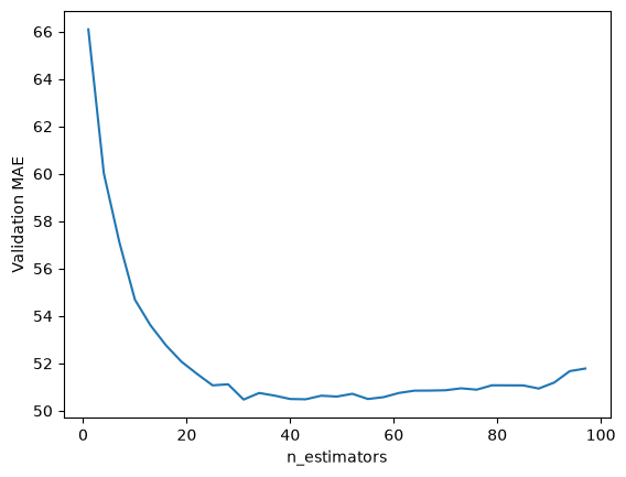
As you can see, the validation error decreases quickly up to about 30 estimators, stays almost flat, and rises slowly after about 60. This behavior must be familiar to you at this point: overfitting! Let’s plot this together with the training error:
n_estimators_list = []
validation_error = []
training_error = []
for n_estimators in range(1, 100, 3):
    gbr = GradientBoostingRegressor(random_state=0, n_estimators=n_estimators)
    gbr.fit(X_train, y_train)
    y_pred = gbr.predict(X_val)
    mae = mean_absolute_error(y_val, y_pred)
    n_estimators_list.append(n_estimators)
    validation_error.append(mae)
    training_error.append(mean_absolute_error(y_train, gbr.predict(X_train)))
plt.plot(n_estimators_list, validation_error, label='validation_error')
plt.plot(n_estimators_list, training_error, label='training_error')
plt.xlabel('n_estimators')
plt.ylabel('MAE')
plt.legend()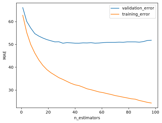
A masterpiece of a plot. We need to understand the hyperparameters next to prevent overfitting.
YOUR TURN
Try GradientBoostingClassifier on the breast cancer dataset. (For reference: with default settings it reaches about 0.96 accuracy in 5-fold cross-validation.)
from sklearn.datasets import load_breast_cancer
# YOUR CODE HERE
3. Hyperparameters
Most hyperparameters will look familiar from decision trees and random forests. Gradient boosting adds a few parameters that control how each tree corrects the errors of the ensemble. Different libraries implement these ideas in slightly different ways, so aim to understand their role conceptually rather than tuning them mechanically. We will cover:
- Learning Rate
- Early Stopping
- Loss
3.1 Learning Rate
Let’s get back to the problem we encountered previously, where adding trees increased the validation error in our initial implementation:
n_estimators = 50
boosted_forest = []
y_residual = y_train.copy()
for i in range(n_estimators):
    dt = DecisionTreeRegressor(random_state=0, max_depth=max_depth)
    dt.fit(X_train, y_residual)
    boosted_forest.append(dt)
    # next iteration
    y_pred = dt.predict(X_train)
    y_residual = y_residual - y_pred

y_pred = sum(dt.predict(X_val) for dt in boosted_forest)
mae = mean_absolute_error(y_val, y_pred)
print("MAE:", mae)
MAE: 61.51269847323992The reason this implementation fails is that we have not included a learning rate. Every tree corrects the remaining errors at full strength. The training error keeps going down, but after a few trees the remaining errors are mostly noise, and each new tree fits that noise as well as it can: the model overfits after a few trees. The key idea is to reduce the influence of each tree by scaling its contribution with a step size, so that every tree adds only a small correction and the model needs more trees to fit the noise. This works exactly like gradient descent and can be implemented as:
y_residual = y_residual - learning_rate * y_predlearning_rate = 0.1 # ADD lr
n_estimators = 50
boosted_forest = []
y_residual = y_train.copy()
for i in range(n_estimators):
dt = DecisionTreeRegressor(random_state=0, max_depth=max_depth)
dt.fit(X_train, y_residual)
boosted_forest.append(dt)
y_pred = dt.predict(X_train)
y_residual = y_residual - learning_rate * y_pred # ADD lr
y_pred = sum(learning_rate * dt.predict(X_val) for dt in boosted_forest) # ADD lr
mae = mean_absolute_error(y_val, y_pred)
print("MAE:", mae)MAE: 50.47766624861128Suddenly the results are much closer to the scikit-learn implementation 🥳🥳 This shows that the core idea behind boosting is conceptually simple, even if production implementations add many refinements.
# learning rate = 1
# this is equal to our initial non-learning rate implementation
learning_rate = 1
n_estimators = 50
boosted_forest = []
y_residual = y_train.copy()
for i in range(n_estimators):
    dt = DecisionTreeRegressor(random_state=0, max_depth=max_depth)
    dt.fit(X_train, y_residual)
    boosted_forest.append(dt)
    y_pred = dt.predict(X_train)
    y_residual = y_residual - learning_rate * y_pred
y_pred = sum(learning_rate * dt.predict(X_val) for dt in boosted_forest)
mae = mean_absolute_error(y_val, y_pred)
print("MAE:", mae)
MAE: 61.51269847323992Now let’s understand the influence of changing the learning rate, by repeating the validation error vs n_estimators plot at different learning rates:
plot_dict = {}

for learning_rate in [0.01, 0.03, 0.1, 0.3, 1]:

    x_for_plotting = []
    y_for_plotting = []
    for n_estimators in range(1, 100, 3):
        gbr = GradientBoostingRegressor(random_state=0, n_estimators=n_estimators, learning_rate=learning_rate)
        gbr.fit(X_train, y_train)
        y_pred = gbr.predict(X_val)
        mae = mean_absolute_error(y_val, y_pred)
        x_for_plotting.append(n_estimators)
        y_for_plotting.append(mae)

    plot_dict[learning_rate] = (x_for_plotting, y_for_plotting)
annotation_location = {0.01: 15, 0.03: -5, 0.1: -5, 0.3: -5, 1: -5}
for lr in plot_dict:
x_vals, y_vals = plot_dict[lr]
plt.plot(x_vals, y_vals)
# annotate lr on the curves
plt.text(x_vals[annotation_location[lr]], y_vals[annotation_location[lr]], f'lr={lr}', fontsize=10, bbox=dict(facecolor='white', alpha=0.6, edgecolor='black'))
plt.xlabel('n_estimators')
plt.ylabel('Validation MAE')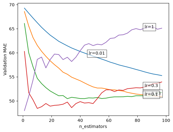
The best way to read this plot is to track how the behavior changes as the learning rate decreases from 1 to 0.01.
- For
lr = 1the error is lowest after the first tree and rises right after it: every tree corrects the remaining errors completely, so the model starts fitting noise right away. - For
lr = 0.3the error drops fast, reaches its minimum after about 10 trees and then rises clearly: with steps this large the model starts to overfit after a few trees. - For
lr = 0.1we get a smooth trajectory with a flat minimum between about 30 and 60 trees. - For
lr = 0.03the error decreases more slowly and reaches the level of thelr = 0.1minimum only at about 100 trees. - For
lr = 0.01the curve looks poor only because we stopped at 100 trees; with more boosting rounds it might reach a better solution.
The validation set has only 45 patients, so differences of one or two MAE between the curves are within the noise: the low point of the lr = 0.3 curve does not prove that 0.3 is the best learning rate. Look at the shapes of the curves rather than at their exact minima.
This illustrates the tradeoff between the learning rate and the number of estimators. Smaller learning rates often lead to better generalization but require more trees and longer training times. These two hyperparameters must be tuned together. Choosing 100 trees for lr = 0.01 leads to underfitting because the model needs many more steps, whereas choosing 100 trees for lr = 0.3 leads to overfitting because each tree corrects too much.
3.2 Early Stopping
The key idea to tune lr and n_estimators together is to use early stopping. Set n_estimators to a large value, monitor the validation error after each tree, and stop when the error starts to rise. However, it is not sensible to stop the moment a single tree increases the error. The curve is not perfectly smooth and small temporary increases can occur even when the overall trend is improving. A better approach is to use patience: allow the model to continue for several more iterations, for example 20, and stop only if the error has not improved during that window. This is called early stopping because training ends before reaching the maximum number of estimators. For this reason it is best to set n_estimators high and rely on early stopping to find the right point. If training actually reaches n_estimators without stopping, the model is likely underfitting, as in the case we have seen above with lr=0.01 and n_estimators=100.
Early stopping watches the validation error, so it needs the validation set that we created at the top of the notebook. The test set plays no part in it.
# let's repeat what we have done
# now we record the validation error after every tree
learning_rate = 0.1
n_estimators = 100
boosted_forest = []
mae_values = []
y_residual = y_train.copy()
for i in range(n_estimators):
    dt = DecisionTreeRegressor(random_state=0, max_depth=max_depth)
    dt.fit(X_train, y_residual)
    boosted_forest.append(dt)
    y_pred = dt.predict(X_train)
    y_residual = y_residual - learning_rate * y_pred

    y_pred = sum(learning_rate * dt.predict(X_val) for dt in boosted_forest)
    mae = mean_absolute_error(y_val, y_pred)
    mae_values.append(mae)
n_estimators_list = list(np.arange(len(mae_values))+1)
plt.plot(n_estimators_list, mae_values)
plt.ylabel('Validation MAE')
plt.xlabel('n_estimators')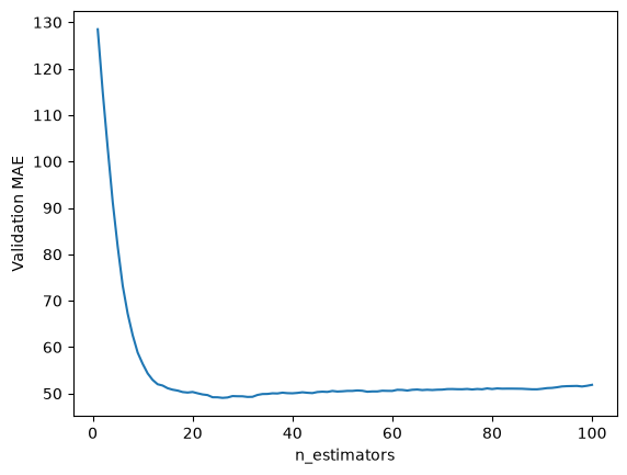
# This is where we want to stop
best_val_mae = min(mae_values)
best_n_estimators = n_estimators_list[mae_values.index(best_val_mae)]

print(f"Best validation MAE: {best_val_mae:.2f}")
print(f"Best n_estimators: {best_n_estimators}")
Best validation MAE: 49.06
Best n_estimators: 26a closer look to the vicinity:
plt.plot(n_estimators_list, mae_values)
plt.xlim(best_n_estimators-15,best_n_estimators+5)
plt.ylim(best_val_mae-1,best_val_mae+5)
plt.scatter(best_n_estimators, best_val_mae, color='red')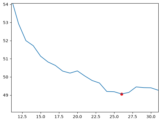
here is how we can add early stopping, changes marked by comments:
learning_rate = 0.1
n_estimators = 500
boosted_forest = []
mae_values = []
y_residual = y_train.copy()

# Addition for early stopping
patience = 20  # num iterations to wait without improvement
best_mae = float("inf") # keep track of the best mae so far
best_iter = -1 # keep track of the best iter so far
no_improve_count = 0 # if this value hits patience we break

for i in range(n_estimators):
    dt = DecisionTreeRegressor(random_state=0, max_depth=max_depth)
    dt.fit(X_train, y_residual)
    boosted_forest.append(dt)
    y_pred_train = dt.predict(X_train)
    y_residual = y_residual - learning_rate * y_pred_train

    y_pred_val = sum(learning_rate * tree.predict(X_val) for tree in boosted_forest)
    mae = mean_absolute_error(y_val, y_pred_val)
    mae_values.append(mae)

    # Addition for early stopping
    if mae < best_mae:
        best_mae = mae
        best_iter = i
        no_improve_count = 0
    else:
        no_improve_count += 1
        if no_improve_count >= patience:
            print(f"Early stopping at iteration {i} with best iteration {best_iter} and MAE={best_mae:.4f}")
            break
Early stopping at iteration 45 with best iteration 25 and MAE=49.0615Keep in mind that when we use early stopping with patience, we do not actually stop at the minimum. Because we use patience, training continues past the optimum and only stops after the model fails to improve for the amount of rounds equal to patience.
# MAE will be higher
y_pred = sum(learning_rate*dt.predict(X_val) for dt in boosted_forest)
mae = mean_absolute_error(y_val, y_pred)
print("MAE:", mae)
MAE: 50.39811062946827so we need to slice the forest until the optimum point:
# keep only the trees up to the best iteration
best_n_estimators = best_iter + 1
boosted_forest = boosted_forest[:best_n_estimators] # slice until the optimum
mae_values = mae_values[:best_n_estimators]

print(f"Using {best_n_estimators} trees with best validation MAE = {best_mae:.4f}")
Using 26 trees with best validation MAE = 49.0615y_pred = sum(learning_rate*dt.predict(X_val) for dt in boosted_forest)
mae = mean_absolute_error(y_val, y_pred)
print("MAE:", mae)MAE: 49.06145405276122The development is finished: we chose the learning rate and the number of trees on the validation set. The final step is to report the test error, once. This is the first time in this notebook that we use the test set.
# Test error
y_pred = sum(learning_rate*dt.predict(X_test) for dt in boosted_forest)
mae = mean_absolute_error(y_test, y_pred)
print("MAE:", mae)
MAE: 44.980923669200933.3 Loss
We mentioned above that the foundations of gradient boosting were laid by Jerome Friedman in 2001 in his paper Greedy Function Approximation: A Gradient Boosting Machine. In the abstract he says:
Function estimation/approximation is viewed from the perspective of numerical optimization in function space, rather than parameter space. A connection is made between stagewise additive expansions and steepest descent minimization. A general gradient descent “boosting” paradigm is developed for additive expansions based on any fitting criterion. Specific algorithms are presented for least-squares, least absolute deviation, and Huber-M loss functions for regression, and multiclass logistic likelihood for classification.
Gradient descent, the optimization method behind many machine learning models, tries to find the best parameters (a search in the parameter space).
\[new\_parameters = old\_parameters − lr × gradient\_of\_the\_loss\_at\_the\_old\_parameters\]
The analogous rule for gradient boosting (the update in function space) becomes:
\[new\_function = old\_function − lr × tree\_that\_approximates\_the\_gradient\_of\_the\_loss\]
How is loss a hyperparameter in our implementation?
learning_rate = 0.1
n_estimators = 100
boosted_forest = []
mae_values = []
y_residual = y_train.copy()
for i in range(n_estimators):
    dt = DecisionTreeRegressor(random_state=0, max_depth=max_depth)
    dt.fit(X_train, y_residual)
    boosted_forest.append(dt)
    y_pred = dt.predict(X_train)

    # HERE IT IS: the new residuals, the negative gradient of the squared-error loss,
    # which the next tree is fitted to
    y_residual = y_residual - learning_rate * y_pred

    y_pred = sum(learning_rate * dt.predict(X_val) for dt in boosted_forest)
    mae = mean_absolute_error(y_val, y_pred)
    mae_values.append(mae)
the loss we implemented is the squared error: the residuals that every tree is fitted to are the negative gradient of the squared error (up to a factor of 2). In scikit-learn this is the default loss. To compare two losses we use 5-fold cross-validation on the development set (X_dev, the training and the validation set together), as in the Modeling and Evaluation notebook: the validation set has only 45 patients, too few to tell two similar models apart, and the test set is not used for comparisons.
from sklearn.model_selection import cross_val_score

gbr = GradientBoostingRegressor(random_state=0, n_estimators=50, loss='squared_error')
scores = -cross_val_score(gbr, X_dev, y_dev, cv=5, scoring='neg_mean_absolute_error')
print(f"MAE: {scores.mean():.1f} ± {scores.std():.1f} (5-fold CV)")
MAE: 45.8 ± 1.4 (5-fold CV)Check the documentation for available loss functions:
loss{‘squared_error’, ‘absolute_error’, ‘huber’, ‘quantile’}, default=’squared_error’
Loss function to be optimized. ‘squared_error’ refers to the squared error for regression. ‘absolute_error’ refers to the absolute error of regression and is a robust loss function. ‘huber’ is a combination of the two. ‘quantile’ allows quantile regression (use alpha to specify the quantile). See Prediction Intervals for Gradient Boosting Regression for an example that demonstrates quantile regression for creating prediction intervals with loss=‘quantile’.
gbr = GradientBoostingRegressor(random_state=0, n_estimators=50, loss='huber')
scores = -cross_val_score(gbr, X_dev, y_dev, cv=5, scoring='neg_mean_absolute_error')
print(f"MAE: {scores.mean():.1f} ± {scores.std():.1f} (5-fold CV)")
MAE: 45.9 ± 1.2 (5-fold CV)The two losses give almost the same cross-validated MAE, so on this data the choice of loss matters little. A robust loss such as huber or absolute_error helps when the targets contain outliers, a few values far from the rest.
4. Popular gradient boosting frameworks
The most popular gradient boosting frameworks are XGBoost, LightGBM and CatBoost. They provide highly optimized implementations of boosting algorithms designed for speed, accuracy and practical use on large datasets. They follow the same core principles while introducing practical advantages. XGBoost is known for strong regularization and dependable performance across many tasks. LightGBM is recognized for very fast training through its histogram based approach and leaf-wise tree growth. CatBoost excels at handling categorical features without manual encoding. All three offer GPU support that can significantly accelerate training. These capabilities have made them widely used in industry and machine learning competitions, and they remain valuable tools for real world predictive modeling.
These three frameworks are already installed in our course environment (see pyproject.toml). On macOS, XGBoost and LightGBM need the OpenMP runtime: if importing them fails, run brew install libomp in a terminal and restart the kernel.
The default model works very similar to scikit-learn:
from xgboost import XGBRegressor

model = XGBRegressor(random_state=0)
model.fit(X_train, y_train)
y_pred = model.predict(X_val)
mae = mean_absolute_error(y_val, y_pred)
print("MAE:", mae)MAE: 54.690865241156686and even most hyperparameters follow the scikit-learn convention:
model = XGBRegressor(random_state=0, max_depth=3, learning_rate=0.1, n_estimators=50)
model.fit(X_train, y_train)
y_pred = model.predict(X_val)
However, there are differences as well. For an overview, please read the documentation:
https://xgboost.readthedocs.io/en/stable/python/python_api.html#xgboost.XGBRegressor
And here you can see a few different use cases for XGBoost in Python.
Now let’s see how early stopping works, at first we can define it as a callback.
A callback is simply a small piece of code that you give to another function so that it can be called back at specific moments during its execution. Think of it as: “While you are training the model, also do this extra thing every time you finish a tree or an epoch.”
# rounds is patience
# save_best is what we did to get the best model rather than best+patience
from xgboost.callback import EarlyStopping
early_stopping = EarlyStopping(rounds=50, save_best=True)
the next step is, when we call the model, provide the early_stopping callback as well as any other hyperparameters. Notice how n_estimators is a large value but the training will stop before that:
model = XGBRegressor(
    random_state=0,
    learning_rate=0.1,
    n_estimators=1000,
    eval_metric='mae',
    callbacks=[early_stopping])
model.fit(
X_train, y_train,
eval_set=[(X_val, y_val)],
verbose=False # no line per tree; the learning curve is plotted below
);XGBoost keeps everything you need for a learning curve inside the trained model.
evals_result = model.evals_result()
evals_result.keys()dict_keys(['validation_0'])mae_vals = evals_result['validation_0']['mae']
n_estimators_list = list(np.arange(len(mae_vals))+1)
plt.plot(n_estimators_list, mae_vals)
plt.ylabel('Validation MAE')
plt.xlabel('n_estimators')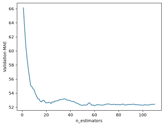
YOUR TURN
CatBoost is also installed in our environment. Visit the CatBoost documentation and train a CatBoostRegressor on the same dataset we have been using in this notebook.
Set verbose=0, otherwise CatBoost prints a line for every tree. (For reference: with default settings, CatBoostRegressor reaches an MAE of about 46 in 5-fold cross-validation on the development set. On the 45 patients of the validation set alone the result varies a lot, so compare models with cross-validation.)
# YOUR CODE HERE5. AdaBoost and Stacking
Gradient boosting is not the only way to boost. AdaBoost, the older method mentioned at the top of this notebook, also trains trees one after the other. Instead of fitting each new tree to the residuals, it gives more weight to the training samples that the previous trees predicted badly, so that the next tree focuses on them. scikit-learn has AdaBoostClassifier and AdaBoostRegressor. Gradient boosting is used more often today, but you will still see AdaBoost in papers and older code.
Stacking combines different models in another way. Several base models make predictions, and a final model learns how to combine those predictions into one. The final model must not learn from predictions that the base models made on their own training data, because those are too good. StackingRegressor therefore trains the final model on cross-validated predictions: each prediction comes from a base model that did not see that sample during training.
We compare them on the development set of this notebook, with 5-fold cross-validation, as the losses in section 3.3. Ridge is the regularized linear regression from the Linear Regression notebook.
from sklearn.dummy import DummyRegressor
from sklearn.ensemble import AdaBoostRegressor, RandomForestRegressor, StackingRegressor
from sklearn.linear_model import Ridge
from sklearn.model_selection import cross_val_score


base_models = [
    ('ridge', Ridge()),
    ('random forest', RandomForestRegressor(random_state=0)),
    ('gradient boosting', GradientBoostingRegressor(random_state=0)),
]
models = {'baseline (mean)': DummyRegressor()} | dict(base_models)
models['AdaBoost'] = AdaBoostRegressor(random_state=0)
models['stacking'] = StackingRegressor(estimators=base_models, final_estimator=Ridge())

for name, model in models.items():
    scores = -cross_val_score(model, X_dev, y_dev, cv=5, scoring='neg_mean_absolute_error')
    print(f"{name:18s} MAE: {scores.mean():.1f} ± {scores.std():.1f} (5-fold CV)")
baseline (mean) MAE: 66.3 ± 3.5 (5-fold CV)
ridge MAE: 49.4 ± 3.1 (5-fold CV)
random forest MAE: 47.0 ± 2.7 (5-fold CV)
gradient boosting MAE: 46.5 ± 2.0 (5-fold CV)
AdaBoost MAE: 47.8 ± 2.6 (5-fold CV)
stacking MAE: 45.5 ± 2.0 (5-fold CV)Every model is far better than the baseline that always predicts the mean (an MAE of 66.3). Stacking has the lowest mean MAE, but all differences between the models are small.
Stacking costs more training time. With the default 5 folds, StackingRegressor trains every base model 6 times: 5 times for the cross-validated predictions and once on all the data, for the predictions on new samples.
Further reading (optional)
- Aurélien Géron, Hands-On Machine Learning with Scikit-Learn, Keras & TensorFlow (O’Reilly), chapter 7, “Ensemble Learning and Random Forests”, from the section on boosting to the end of the chapter.
- James et al., An Introduction to Statistical Learning with Applications in Python (free to read online), chapter 8, section 8.2 on boosting.